
Hold on.
Hold on.
Wait.
You’re telling me, that combining independently sampled data into a single pool, from independent sources, can provide assumptions as it pertains to the source of each sample?
Yes!
And this methodology provides a better estimator than other available conventional methods?
Yes again.
This was the conversation which divided the math world in 1956.
Here is an article detailing the phenomenon and findings of Charles Steins from Scientific America (.PDF Warning):
https://efron.ckirby.su.domains//other/Article1977.pdf
Since we have computers, let’s give the James-Stein’s Estimator a little test-er-roo. In the digital era, we are no longer forced to accept hearsay proofs.
(The code below is a heavily modified and simplified version of code which was originally queried from: https://bookdown.org/content/922/james-stein.html)
##################################################################################
### Stein’s Paradox / The James-Stein Estimator ###
## We begin by creating 5 independent samples generated from normally distributed data sources ##
## Each sample is comprised of random numbers ##
# 100 Random Numbers, Mean = 500, Standard Deviation = 155 #
Ran_A <- rnorm(100, mean=500, sd=155)
# 100 Random Numbers, Mean = 50, Standard Deviation = 22 #
Ran_B <- rnorm(100, mean=50, sd= 22)
# 100 Random Numbers, Mean = 1, Standard Deviation = 2 #
Ran_C <- rnorm(100, mean=1, sd = 2)
# 100 Random Numbers, Mean = 1000, Standard Deviation = 400 #
Ran_D <- rnorm(100, mean=1000, sd=400)
# I went ahead and sampled a few of the elements from each series which were generated by my system #
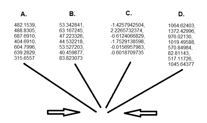
testA <- c(482.154, 488.831, 687.691, 404.691, 604.8, 639.283, 315.656)
testB <- c(53.342841, 63.167245, 47.223326, 44.532218, 53.527203, 40.459877, 83.823073)
testC <-c(-1.4257942504, 2.2265732374, -0.6124066829, -1.7529138598, -0.0156957983, -0.6018709735 )
testD <- c(1064.62403, 1372.42996, 976.02130, 1019.49588, 570.84984, 82.81143, 517.11726, 1045.64377)
# We now must create a series which contains all of the sample elements #
testall <- c(testA, testB, testC, testD)
# Then we will take the mean measurement of each sampled series #
MLEA <- mean(testA)
MLEB <- mean(testB)
MLEC <- mean(testC)
MLED <- mean(testD)
# Next, we will derive the mean of the combined sample elements #
p_ <- mean(testall)
# We must assign to ‘N’, the number of sets which we are assessing #
N <- 4
# We must also derive the median of the combined sample elements #
medianden <- median(testall)
# Sigma2 = mean(testall) * (1 – (mean(testall)) / medianden #
sigma2 <- p_ * (1-p_) / medianden
# Now we’re prepared to calculate the assumed population mean of each sample series #
c_A <- p_+(1-((N-3)*sigma2/(sum((MLEA-p_)^2))))*(MLEA-p_)
c_B <- p_+(1-((N-3)*sigma2/(sum((MLEB-p_)^2))))*(MLEB-p_)
c_C <- p_+(1-((N-3)*sigma2/(sum((MLEC-p_)^2))))*(MLEC-p_)
c_D <- p_+(1-((N-3)*sigma2/(sum((MLED-p_)^2))))*(MLED-p_)
##################################################################################
# Predictive Squared Error #
PSE1 <- (c_A - 500) ^ 2 + (c_B - 50) ^ 2 + (c_C - 1) ^ 2 + (c_D - 1000) ^ 2
########################
# Predictive Squared Error #
PSE2 <- (MLEA- 500) ^ 2 + (MLEB - 50) ^ 2 + (MLEC - 1) ^ 2 + (MLED - 1000) ^ 2
########################
1 - 28521.5 / 28856.74
##################################################################################
1 - 28521.5 / 28856.74 = 0.01161739
So, we can conclude, through the utilization of MSE as an accuracy assessment technique, that Stein’s Methodology (AKA The James-Stein Estimator), provided a 1.16% better estimation of the population mean for each series, as compared to the mean of each sample series assessed independently.
Charles Stein really was a pioneer in the field of statistics as he discovered one of the first instances of dimension reduction.
If we consider our example data sources below:
Charles Stein really was a pioneer in the field of statistics as he discovered one of the first instances of dimension reduction.
If we consider our example data sources below:

Series elements which were already in close proximity to the mean, now move slightly closer to the mean. Series elements which were originally far from the mean, move much closer to the mean. These outside elements still maintain their order, but they are brought closer to their fellow series peers. This shifting of the more extreme elements within a series, is what makes the James-Stein Estimator so novel in design, and potent in application.
This one really blew my noggin when I first discovered and applied it.
For more information on this noggin blowing technique, please check out:
https://www.youtube.com/watch?v=cUqoHQDinCM
That's all for today.
Come back again soon for more perspective altering articles.
-RD