(Python) The Number: 13 (Happy, Lucky, Primes) - A Spooky Special!

This Halloween, we’ll be covering a very spooky topic. 

I feel that the number “13”, for far too long, has been un-fairly maligned.

Today, it will have its redemption.

Did you know that the number “13”, by some definitions, is both a happy and lucky number? Let’s delve deeper into each definition, and together discover why this number deserves much more respect than it currently receives.

Happy Numbers
 
In number theory, a happy number is a number which eventually reaches 1 when replaced by the sum of the square of each digit. * 

Example:   

For instance, 13 is a happy number because:

(1 * 1) + (3 * 3) = 10

(1 * 1) + (0 * 0) = 1

and the number 19 is also a happy number because:

(1 * 1) + (9 * 9) = 82

(8 * 8) + (2 * 2) = 68

(6 * 6) + (8 * 8) = 100

(1 * 1) + (0 * 0) + (0 * 0) = 1

*- https://en.wikipedia.org/wiki/Happy_number

Lucky Numbers

In number theory, a lucky number is a natural number in a set which is generated by a certain "sieve". *

In the case of our (lucky) number generation process, we will be utilizing the, "the sieve of Josephus Flavius".

Example:

Beginning with a list of integers from 1 – 20:

{1, 2, 3, 4, 5, 6, 7, 8, 9, 10, 11, 12, 13, 14, 15, 16, 17, 18, 19, 20}

We will remove all even numbers:

1, 2, 3, 4, 5, 6, 7, 8, 9, 10, 11, 12, 13, 14, 15, 16, 17, 18, 19, 20

Leaving:

1, 3, 5, 7, 9, 11, 13, 15, 17, 19

The first remaining number after the number “1”, is the number “3”. Therefore, every third number within the list must be removed:

1, 3, 5, 7, 9, 11, 13, 15, 17, 19

Leaving:

1, 3, 7, 9, 13, 15, 19

Next, we will remove each seventh entry within the remaining list, as the number “7” is the value which occurs subsequent to “3”:

1, 3, 7, 9, 13, 15, 19

Leaving:

1, 3, 7, 9, 13, 15

If we were to continue with this process, each ninth entry which would also be subsequently removed from the remaining list, as the number “9” is the number which occurs subsequent to “7”. Since only 6 elements remain from our initial set, the process ends here.

We can then conclude, that the following numbers are indeed lucky:

1, 3, 7, 9, 13, 15

*- https://en.wikipedia.org/wiki/Lucky_number 

Prime Numbers

A prime number is a natural number greater than 1 that is not a product of two smaller natural numbers. *

13 fits this categorization, as it can only be factored down to a product of 13 and 1.

*- https://en.wikipedia.org/wiki/Prime_number

(Python) Automating the Process

Now that I have hopefully explained each concept in an understandable way, let’s automate some of these processes.

Happy Numbers

# Create a list of happy numbers between 1 and 100 #

# https://en.wikipedia.org/wiki/Happy_number #

# This code is a modified variation of the code found at: #

# https://www.phptpoint.com/python-program-to-print-all-happy-numbers-between-1-and-100/ #

# Python program to print all happy numbers between 1 and 100 #


# isHappyNumber() will determine whether a number is happy or not #

def isHappyNumber(num):

    rem = sum = 0;


# Calculates the sum of squares of digits #

    while(num > 0):

        rem = num%10;

        sum = sum + (rem*rem);

        num = num//10;

    return sum;


# Displays all happy numbers between 1 and 100 #     

print("List of happy numbers between 1 and 100: \n 1");



# for i in range(1, 101):, always utilize n+1 as it pertains to the number of element entries within the set #

# Therefore, for our 100 elements, we will utilize 101 as the range variable entry #


for i in range(1, 101):

    result = i;

    while(result != 1 and result != 4):

        result = isHappyNumber(result);

        if(result == 1):

            print(i);


Console Output:

List of happy numbers between 1 and 100:
1
7
10
13
19
23
28
31
32
44
49
68
70
79
82
86
91
94
97
100

# Code which verifies whether a number is a happy number #

# Code Source: # https://en.wikipedia.org/wiki/Happy_number #

# This process is unfortunately two steps # 

def pdi_function(number, base: int = 10):

    """Perfect digital invariant function."""

    total = 0

    while number > 0:

        total += pow(number % base, 2)

        number = number // base

return total


def is_happy(number: int) -> bool:

    """Determine if the specified number is a happy number."""

    seen_numbers = set()

    while number > 1 and number not in seen_numbers:

        seen_numbers.add(number)

        number = pdi_function(number)

    return number == 1


# First, we must run the initial function on the number in question #

# This function will calculate the number’s perfect digital invariant value #

# Example, for 13 #

pdi_function(13)

Console Output:

10

# The output value of the first function must then be input into the subsequent function, in order to determine whether or not the tested value (ex. 13) can appropriately be deemed “happy”. #

is_happy(10)

Console Output:

True

Lucky Numbers

# https://en.wikipedia.org/wiki/Lucky_number #

# The code below will determine whether or not a number is "lucky", as defined by the above definition of the term #

# The variable ‘number check’, must be set equal to the number which we wish to assess  #

number_check = 99


# Python code to convert list of #

# string into sorted list of integer #

# https://www.geeksforgeeks.org/python-program-to-convert-list-of-integer-to-list-of-string/ #


# List initialization

list_int = list(range(1,(number_check + 1),1))


# mapping

list_string = map(str, list_int)


# Printing sorted list of integers

numbers = (list(list_string))


# https://stackoverflow.com/questions/64956140/lucky-numbers-in-python #


def lucky_numbers(numbers):

    index = 1

    next_freq = int(numbers[index])

    while int(next_freq) < len(numbers):

        del numbers[next_freq-1::next_freq]

        print(numbers)

        if str(next_freq) in numbers:

            index += 1

            next_freq = int(numbers[index])

else:

    next_freq = int(numbers[index])

return


lucky_numbers(numbers)


Console Output:

['1', '3', '5', '7', '9', '11', '13', '15', '17', '19', '21', '23', '25', '27', '29', '31', '33', '35', '37', '39', '41', '43', '45', '47', '49', '51', '53', '55', '57', '59', '61', '63', '65', '67', '69', '71', '73', '75', '77', '79', '81', '83', '85', '87', '89', '91', '93', '95', '97', '99']

['1', '3', '7', '9', '13', '15', '19', '21', '25', '27', '31', '33', '37', '39', '43', '45', '49', '51', '55', '57', '61', '63', '67', '69', '73', '75', '79', '81', '85', '87', '91', '93', '97', '99']

['1', '3', '7', '9', '13', '15', '21', '25', '27', '31', '33', '37', '43', '45', '49', '51', '55', '57', '63', '67', '69', '73', '75', '79', '85', '87', '91', '93', '97', '99']

['1', '3', '7', '9', '13', '15', '21', '25', '31', '33', '37', '43', '45', '49', '51', '55', '63', '67', '69', '73', '75', '79', '85', '87', '93', '97', '99']

['1', '3', '7', '9', '13', '15', '21', '25', '31', '33', '37', '43', '49', '51', '55', '63', '67', '69', '73', '75', '79', '85', '87', '93', '99']

['1', '3', '7', '9', '13', '15', '21', '25', '31', '33', '37', '43', '49', '51', '63', '67', '69', '73', '75', '79', '85', '87', '93', '99'] 

The output of this function returns a series of numbers up to and including the number which is being assessed. Therefore, from this function's application, we can conclude that the following numbers are "lucky":

['1', '3', '7', '9', '13', '15', '21', '25', '31', '33', '37', '43', '49', '51', '63', '67', '69', '73', '75', '79', '85', '87', '93', '99'] 

(Only consider the final output as valid, as all other outputs are generated throughout the reduction process)

Prime Numbers

# The code below is rather self-explanatory #

# It is utilized to generate a a list of prime numbers included within the range() function # 

# Source: https://stackoverflow.com/questions/52821002/trying-to-get-all-prime-numbers-in-an-array-in-python #

checkMe = range(1, 100)

primes = []

for y in checkMe[1:]:

    x = y

    dividers = []

    for x in range(2, x):

        if (y/x).is_integer():

            dividers.append(x)

if len(dividers) < 1:
    
    primes.append(y)

print("\n"+str(checkMe)+" has "+str(len(primes))+" primes")

print(primes)

Console Output:

range(1, 100) has 25 primes
[2, 3, 5, 7, 11, 13, 17, 19, 23, 29, 31, 37, 41, 43, 47, 53, 59, 61, 67, 71, 73, 79, 83, 89, 97]

Conclusion

Having performed all of the previously mentioned tests and functions, I hope that you have been provided with enough adequate information to reconsider 13's unlucky status. Based upon my number theory research, I feel that enough evidence exists to at least relegate the number 13 to the status of "misunderstood".

13 isn't to be feared or avoided. It actually shares unique company amongst other "Happy Primes":

7, 13, 19, 23, 31, 79, 97, 103, 109, 139, 167, 193, 239, 263, 293, 313, 331, 367, 379, 383, 397, 409, 487

Even intermingling with the company of "Lucky Primes":

3, 7, 13, 31, 37, 43, 67, 73, 79, 127, 151, 163, 193, 211, 223, 241, 283, 307, 331, 349, 367, 409, 421, 433, 463, 487

And being a member of the very exclusive group, the "Happy Lucky Primes":

7, 13, 31, 79, 193, 331, 367, 409, 487

----------------------------------------------------------------------------------------------------------------------------- 

I wish you all a very happy and safe holiday.

I'll see you next week with more (non-spooky) content!

-RD

(Python) Machine Learning – Keras – Pt. V

Throughout the previous articles, we thoroughly explored the various machine learning techniques which employ tree methodologies as their primary mechanism. We also discussed the evolution of machine learning techniques, and how gradient boosting eventually came to overtake the various forest models as the preferred standard. However, the gradient boosted model was soon replaced by the Keras model. The latter still remains the primary method of prediction at this present time.

Keras differs from all of the other models in that it does not utilize the tree or forest methodologies as its primary mechanism of prediction. Instead, Keras employs something similar to a binary categorical method, in that, an observation is fed through the model, and at each subsequent layer prior to the output, Keras decides what the observation is, and what the observation is not. This may sound somewhat complicated, and in all manners, it truly is. However, what I am attempting to illustrate will become less opaque as you continue along with the exercise.

A final note prior to delving any further, Keras is a member of a machine learning family known as deep learning. Deep learning can essentially be defined as an algorithmic analysis of data which can evaluate non-linear relationships. This analysis also provides dynamic model re-calibration throughout the modeling process.

Keras Illustrated

Below is a sample illustration of a Keras model which possesses a continuous dependent variable. The series of rows on the left represents the observational data which will be sent through the model so that it may “learn”. Each circle represents what is known as “neuron”, and each column of circles represents what is known as a “layer”. The sample illustration has 4 layers. The leftmost layer is known as the input layer, the middle two layers are known as the hidden layers, and the rightmost layer is referred to as the output layer.

Due to the model’s continuous dependent variable classification, it will only possess a single output layer. If the dependent variable was categorical, it would have an appearance similar to the graphic below:

How the Model Works

Without getting overly specific, (as many other resources exist which provide detailed explanations as it pertains the model’s inner-most mechanisms), the training of the model occurs throughout two steps. The first step being: “Forward Propagation”, and the second step being: “Backward Propagation”. Each node which exists beyond the input layers, sans the output layer, is measuring for a potential interaction amongst variables.

Each node is initially assigned a value. Those values shift as training data is processed through the model from the left to the right (forward propagation), and further, but more specifically modified, as the same data is then passed back through the model from the right to the left (back propagation). The entire training data set is not processed in its entirety in a simultaneous manner, instead, for the sake of allocating computing resources, the data is split into smaller sets known as batches. Batch size impacts learning significantly. With a smaller batch size, a model’s predictive capacity will be hindered. However, there are certain scenarios when lower batch size is advantageous, as the impact of noisy gradients will be reduced. The default size for a batch is 32 observations.

In many ways, the method in which the model functions is analogous to the way in which a clock operates. Each training observation shifts a certain aspect of a neuron’s value, with the neuron’s final value being representational of all of the prior shifts.

A few other terms which are also worth mentioning, as the selection of such is integral to model creation are:

Optimizer – This specifies the algorithm which will be utilized for correcting the model as errors occur.

Epoch – This indicates the number of times in which observational data will be passed through a model during the training process.

Loss Function – This indicates the algorithm which will be utilized to determine how errors are penalized within the model.

Metric - A metric is a function which is utilized to assess the performance of a model. However, unlike the Loss Function, it does not impact model training, and is only utilized to perform post-hoc analysis.

Model Application

As with any auxiliary python library, a library must first be downloaded and enabled prior to its utilization. To achieve this within the Jupyter Notebook platform, we will employ the following lines of code:

# Import ‘pip’ to import to install auxiliary packages #

import pip

# Install ‘TensorFlow’ to act as the underlying mechanism of the Keras UI #

pip.main(['install', 'TensorFlow'])

# Import pandas to enable data frame utilization #

import pandas

# Import numpy to enable numpy array utilization #

import numpy

# Import the general Keras library #

import keras

# Import tensorflow to act as the ‘backend’ #

import tensorflow

# Enable option for categorical analysis #

from keras.utils import to_categorical

from keras.models import Sequential

from keras.layers import Activation, Dense

# Import package to enable confusion matrix creation #

from sklearn.metrics import confusion_matrix

# Enable the ability to save and load models with the ‘load_model’ option #

from keras.models import load_model

# Enable the creation of confusion matrixes with the ‘sklearn.metrics’ library #

from sklearn.metrics import confusion_matrix

With all of the appropriate libraries downloaded and enabled, we can begin building our sample model.

Categorical Dependent Variable Model

For the following examples, we will be utilizing a familiar data set, the “iris” data set, which is available within the R platform.

# Import the data set (in .csv format), as a pandas data frame #

filepath = "C:\\Users\\Username\\Desktop\\iris.csv"

iris = pandas.read_csv(filepath)

First we will randomize the observations within the data set. Observational data should always be randomized prior to model creation.

# Shuffle the data frame #

iris = iris.sample(frac=1).reset_index(drop=True)

Next, we will remove the dependent variable entries from the data frame and modify the structure of the new data frame to consist only of independent variables.

predictors = iris.drop(['Species'], axis = 1).as_matrix()

Once this has been achieved, we must modify the variables contained within the original data set so that the categorical outcomes are designated by integer values.

This can be achieved through the utilization of the following code:

# Modify the dependent variable so that each entry is replaced with a corresponding integer #

from pandasql import *

pysqldf = lambda q: sqldf(q, globals())

q = """

SELECT *,

CASE

WHEN (Species = 'setosa') THEN '0'

WHEN (Species = 'versicolor') THEN '1'

WHEN (Species = 'virginica') THEN '2'

ELSE 'UNKNOWN' END AS SpeciesNum

from iris;

"""

df = pysqldf(q)

print(df)

iris0 = df

Next, we must make a few further modifications.

First, we must modify the dependent variable type to integer.

After such, we will identify this variable as being representative of a categorical outcome.

# Modify the dependent variable type from string to integer #

iris0['SpeciesNum'] = iris0['SpeciesNum'].astype('int')

# Modify the variable type to categorical #

target = to_categorical(iris0.SpeciesNum)

We are now ready to build our model!

# We must first specify the model type #

model = Sequential()

# Next, we will specify the output dimensions. This value will typically be [1] unless you are working with images. #

n_cols = predictors.shape[1]

# This next line specifies the traits of the input layer #

model.add(Dense(100, activation = 'relu', input_shape = (n_cols, )))

# This line specifies the traits of the hidden layer #

model.add(Dense(100, activation = 'relu'))

# This line specifies the traits of the output layer #

model.add(Dense(3, activation = 'softmax'))

# Compile the model by adding the optimizer, the loss function type, and the metric type #

# If the model’s dependent variable is binary, utilize the ‘binary_crossentropy' loss function #

model.compile(optimizer = 'adam', loss='categorical_crossentropy',

metrics = ['accuracy'])

With our model created, we can now go about training it with the necessary information.

As was the case with prior machine learning techniques, only a portion of the original data frame will be utilized to train the mode.

model.fit(predictors[1:100,], target[1:100,], shuffle=True, batch_size= 50, epochs=100)

With the model created, we can now test its effectiveness by applying it to the remaining data observations.

# Create a data frame to store the un-utilized observational data #

iristestdata = iris0[101:150]

# Create a data frame to store the model predictions for the un-utilized observational data #

predictions = model.predict_classes(predictors[101:150])

# Create a confusion matrix to assess the model’s predictive capacity #

cm = confusion_matrix(iristestdata['SpeciesNum'], predictions)

# Print the confusion matrix results to the console output window #

print(cm)

Console Output:

[[16    0    0]
[    0  17    2]
[    0    0   14]] 

Continuous Dependent Variable Model

The utilization of differing model types is necessitated by the scenario that each situation dictates. As was the case with previous machine learning methodologies, the Keras package also contains functionality which allows for continuous dependent variables types.

The steps for applying this model methodology are as follows:

# Import the 'iris' data frame #

filepath = "C:\\Users\\Username\\Desktop\\iris.csv"

iris = pandas.read_csv(filepath)

# Shuffle the data frame #

iris = iris.sample(frac=1).reset_index(drop=True)

In the subsequent lines of code, we will first identify the model’s dependent variable ‘Sepal.Length’. This variable, and its corresponding observations will be held within the new variable ‘iris0’. Next, we will create the variable, ‘predictors’. This variable will be comprised of all of the variables contained within the ‘iris0’ data frame, with the exception of the ‘Sepal.Length’ variable. The new data frame will stored within a matrix format. Finally, we will again define the ‘n_cols’ variable.

target = iris['Sepal.Length']

# Drop Species Name #

iris0 = iris.drop(columns=['Species'])



# Drop Species Name #

predictors = iris0.drop(['Sepal.Length'], axis = 1).as_matrix()

n_cols = predictors.shape[1]

We are now ready to build our model!

# We must first specify the model type #

modela = Sequential()

# Next, we will specify the output dimensions. This value will typically be [1] unless you are working with images. #

n_cols = predictors.shape[1]

# This next line specifies the traits of the input layer #

modela.add(Dense(100, activation = 'relu', input_shape=(n_cols,)))

# This line specifies the traits of the hidden layer #

modela.add(Dense(100, activation = 'relu'))

# This line specifies the traits of the output layer #

modela.add(Dense(1))

# Compile the model by adding the optimizer and the loss function type #

modela.compile(optimizer = 'adam', loss='mean_squared_error')

With the model created, we must now train the model with the following code:

modela.fit(predictors[1:100,], target[1:100,], shuffle=True, epochs=100)

As was the case with the prior examples, we will only be utilizing a sample of the original data frame for the purposes of model training.

With the model created and trained, we can now test its effectiveness by applying it to the remaining data observations.

from sklearn.metrics import mean_squared_error

from math import sqrt

predictions = modela.predict(predictors)

rms = sqrt(mean_squared_error(target, predictions))

print(rms)

Model Functionality

In some ways, the Keras modeling methodology shares similarities with the hierarchal cluster model. The main differentiating factor being, in addition to the underlying mechanism, the dynamic aspects of the Keras model.

Each Keras neuron represents a relationship between independent data variables within the training set. These relationships exhibit macro phenomenon which may not be immediately observable within the context of the initial data. When finally providing an output, the model considers which macro phenomenon illustrated the strongest indication of identification. The Keras model still relies on generalities to make predictions, therefore, certain factors which are exhibited within the observational relationships are held in higher regard. This phenomenon is known as weighing, as each neuron is assigned a weight which is adjusted as the training process occurs.

The logistic regression methodology functions in a similar manner as it pertains to assessing variable significance. Again however, we must consider the many differentiating attributes of each model. In addition to weighing latent variable phenomenon, the Keras model is able to assess for non-linear relationships. Both attributes are absent within the aforementioned model, as logistic regression only assesses for linear relationships and can only provide values for variables explicitly found within the initial data set.

The sequential() model type, which was specified within the build process, is one of the many model options available within the Keras package. The sequential option differs from the other model types in that it creates a network in which each neuron within each layer, is connected to each neuron within each subsequent layer. 

 Other Characteristics of the Keras Model

Depending on the size of the data set which acted as the training data for the model, significant time may be required to re-generate a model after a session is terminated. To avoid this un-necessary re-generation process, functions exist which enable the saving and reloading of model information.

# Saving and Loading Model Data Requires #

from keras.models import load_model

# To save a model #

modelname.save("C:\\Users\\filename.h5")

# To load a model #

modelname = load_model("C:\\Users\\filename.h5")

It should be mentioned that as it pertains to Keras models, you do possess the ability to train existing models with additional data should the need the arise.

For instance, if we wished to train our categorical iris model (“model”) with additional iris data, we could utilize the following code:

model.fit(newpredictors[100:150,], newtargets[100:150,], shuffle=True, batch_size= 50, epochs=100)

There are errors which currently exist at the time of this article’s creation, which have yet to be resolved pertaining to learning rate fluctuation within re-loaded Keras models. Currently, a provisional fix has been suggested*, in which the "adam" optimizer is re-configured for re-loaded models. This re-configuring, while keeping all of the "adam" optimizer default configurations, significantly lowers the optimizer’s default learning rate. The purpose of this shift is to account for the differentiation in learning rates which occur in established models.

# Specifying Optimizer Traits Requires #

from keras import optimizers

# Re-configure Optimizer #

liladam = optimizers.adam(lr=0.00001, beta_1=0.9, beta_2=0.999, epsilon=None, decay=0.0, amsgrad=False)

# Utilize Custom Optimizer #

model.compile(optimizer = liladam, loss='categorical_crossentropy',

            metrics = ['accuracy'])

*Source - https://github.com/keras-team/keras/issues/2378

Graphing Models

As we cannot easily determine the innermost workings of a Keras model, the best method of visualization can be achieved by graphing the learning output.

Prior to training the model, we will modify the typical fitting function to resemble something similar to the lines of code below:

history = model.fit(predictors[1:100,], target[1:100,], shuffle=True, epochs= 110, batch_size = 100, validation_data =(predictors[100:150,] , target[100:150,]))

What this code enables, is the creation of the data variable “history”, in which, data pertaining to the model training process will be stored. “validation_data” is instructing the python library to assess the specified data within the context of the model after each epoch. This does not impact the learning process. The way in which this assessment will be analyzed is determined by the selection of the “meteric” option specified within the model.fit() function.

If the above code is initiated, the model will be trained. To view the categories in which the model training history was organized upon being saved within the “history” variable, you may utilize the following lines of code.

history_dict = history.history

history_dict.keys()

This produces the console output:

dict_keys(['val_loss', 'val_acc', 'loss', 'acc'])

To set the appropriate axis lengths for our soon to be produced graph, we will initiate the following line:

epochs = range(1, len(history.history['acc']) + 1)

If we are utilizing Jupyter Notebook, we should also modify the graphic output size:

plt.rcParams["figure.figsize"] = [16,9]

We are now prepared to create our outputs. The first graphic can be prepared with the following code:

# Plot training & validation accuracy values #

# (This graphic cannot be utilized to track the validation process of continuous data models) #

plt.plot(epochs, history.history['acc'], 'b', label = 'Training acc')

plt.plot(epochs, history.history['val_acc'], 'bo', color = 'orange', label = 'Validation acc')

plt.title('Training and validation accuracy')

plt.ylabel('Loss')

plt.xlabel('Epoch')

plt.legend(loc='upper left')

plt.show()

This produces the output:

Interpreting this Graphic

What this graphic is illustrating, is the level of accuracy in which the model predicts results. The solid blue line represents the data which was utilized to train the model, and the orange dotted line represents the data which is being utilized to test the model’s predictability. It should be evident that throughout the training process, the predictive capacity of the model improves as it pertains to both training and validation data. If a large gap emerged, similar to the gap which is observed from epoch # 20 to epoch # 40, we would assume that this divergence of data is indicative of “overfitting”. This term is utilized to describe a model which can predict training results accurately, but struggles to predict outcomes when applied to new data.

The second graphic can be prepared with the following code:

# Plot training & validation loss values

plt.plot(epochs, history.history['loss'], 'b', label = 'Training loss')

plt.plot(epochs, history.history['val_loss'], 'bo', label = 'Validation loss', color = 'orange')

plt.title('Training and validation loss')

plt.ylabel('Loss')

plt.xlabel('Epoch')

plt.legend(loc='upper left')

plt.show()

Interpreting this Graphic

This graphic is illustrates the improvement of the model over time. The solid blue line represents the data which was utilized to train the model, and the orange dotted line represents the data which is being utilized to test the model’s predictability. If a gap does not emerge between the lines throughout the training process, it is advisable to set the number of epochs to a figure which, after subsequent graphing occurs, demonstrates a flat plateauing of both lines.

Reproducing Model Training Results

If Keras is being utilized, and TensorFlow is the methodology selected to act as a “backend”, then the following lines of code must be utilized to guarantee reproductivity of results.

# Any number could be utilized within each function #

# Initiate the RNG of the general python library #

import random

# Initiate the RNG of the numpy package #

import numpy.random

# Set a random seed as it pertains to the general python library #

random.seed(777)

# Set a random seed as it pertains to the numpy library #

numpy.random.seed(777)

# Initiate the RNG of the tensorflow package #

from tensorflow import set_random_seed

# Set a random seed as it pertains to the tensorflow library #

set_random_seed(777)

Missing Values in Keras

Much like the previous models discussed, Keras has difficulties as it relates to variables which contain missing observational values. If a Keras model is trained on data which contains missing variable values, the training process will occur without interruption, however, the missing values will be analyzed under the assumption that they are representative of a measurement. Meaning, that the library will NOT automatically assume that the value is a missing value, and from such, estimate a place holder value based on other variable observations within the set.

To make assumptions for the missing values based on the process described above, we must utilize the imputer() function from the python library: “sklearn”. Sample code which can be utilized for this purpose can be found below:

from sklearn.preprocessing import Imputer

imputer = Imputer()

transformed_values = imputer.fit_transform(predictors)

Additional details pertaining to this function, its utilization, and its underlying methodology, can be found within the previous article: “(R) Machine Learning - The Random Forest Model – Pt. III”.

Having tested this method of variable generation on sets which I purposely modified, I can attest that its capability for achieving such is excellent. After generating fictitious placeholder values and then subsequently utilizing the Keras package to create a model, comparatively speaking, I saw no differentiation between the predicted results related to each individual set.

Early Stopping

There may be instances which necessitate the creation of a model that will be applicable to a very large data set. This essentially, in most cases, guarantees a very long training time. To help assist in shortening this process, we can utilize an “early stopping monitor”.

First, we must import the package related to this feature:

from keras import losses

Next we will create and define the parameters pertaining to the feature:

# If model improvement stagnates after 2 epochs, the fitting process will cease #

early_stopping_monitor = keras.callbacks.EarlyStopping(monitor='loss', patience = 2, min_delta=0, verbose=0, mode='auto', baseline=None, restore_best_weights=True)

Many of the options present within the code above are defaults. However, there are few worth mentioning.

monitor = ‘loss’ - This option is specifically instructing the function to monitor the loss value during each training epoch.

patience = 2 – This option is instructing the function to cease training if the loss value ceases to decline after 2 epochs.

restore_best_weights=True – This option is indicating to the function that the values which occurred prior to lack of loss within the training process, should be the last values applied as it pertains to model training. The subsequent training values will be discarded.

With the early stopping feature defined, we can add it to the training function below:

history = model.fit(predictors[101:150,], target[101:150,], shuffle=True, epochs=100, callbacks =[early_stopping_monitor], validation_data =(predictors[100:150,] , target[100:150,]))

Final Thoughts on Keras

In my final thoughts pertaining to the Keras model, I would like to discuss the pros and cons of the methodology. Keras is, without doubt, the machine learning model type which possesses the greatest predictive capacity. Keras can also be utilized to identify images, which is a feature that is lacking within most other predive models. However, despite these accolades, Keras does fall short in a few categories.

For one, the mathematics which act a mechanism for the model’s predicative capacity are incredibly complex. As a result of such, model creation can only occur within a digital medium. With this complexity comes an inability to easily verify or reproduce results. Additionally, creating the optimal model configuration as it pertains to the number of neurons, layers, epochs, etc., becomes almost a matter of personal taste. This sort of heuristic approach is negative for the field of machine learning, statistics, and science in general.

Another potential flaw relates to the package documentation. The website for the package is poorly organized. The videos created by researchers who attempt to provide instruction are also poorly organized, riddled with heuristic approach, and scuttled by a severe lack of awareness. It would seem that no single individual truly understands how to appropriately utilize all of the features of the Keras package. In my attempts to properly understand and learn the Keras package, I purchased the book, DEEP LEARNING with Python, written by the package’s creator, Francois Chollet. This book was also poorly organized, and suffered from the assumption that the reader could inherently understand the writer’s thoughts.

This being said, I do believe that the future of statistics and predictive analytics lies parallel with the innovations demonstrated within the Keras package. However, the package is so relatively new, that not a single individual, including the creator, has had the opportunity to utilize and document its potential. In this lies latent opportunity for the patient individual to prosper by pioneering the sparse landscape.

It is my opinion that at this current time, the application of the Keras model should be paired with other traditional statistical and machine learning methodologies. This pairing of multiple models will enable the user and potential outside researchers to gain a greater understanding as to what may be motivating the Keras model’s predictive outputs.

(R) Machine Learning - Gradient Boosted Algorithms – Pt. IV

Of all the models which have been discussed thus far, the most complicated, and the most effective of the models which utilize the tree methodology, are the models which belong to a primary sub-group known as, “gradient boosted algorithms”.

Gradient boosted models are similar to the random forest model, the primary difference between the two is that the gradient boosted models synthesize their individual trees differently. Whereas random forests seek to minimize errors through a randomization process, gradient boosted models address each incorrect model within each tree as it is created. Meaning, that each tree is re-assessed after its creation occurs, and the subsequent tree is optimized based on acknowledgement of the prior tree’s errors.

Model Creation Options

As the gradient boosted algorithm possesses components of all of the previously discussed model methodologies, the complexities of the algorithm’s internal mechanism are evident by design. In essence, the evolved capacity of the model, possessing various foundational elements which were initially designated as aspects of prior methodologies, ultimately, through various stages of synthesis, produces a model with a greater number of options. These options can remain at their default assignments in which they were initially designated. As such, they will assume predetermined values in accordance to the surrounding circumstances. However, if you would like to customize the model’s synthesis, the following options are available for such:

distribution – This option refers to the distribution type which the model will assume when analyzing the data utilized within the model design process. The following distribution types are available within the “gbm” package: “gaussian”, “laplace”, “tdist”, “bernoulli”, “huberized”, “adaboost”, “poisson”, “coph”, “quantile” and “pairwise”. If this option is not explicitly indicated by the user, they system will automatically decide between “gaussian” and “bernoulli”, as to which distribution type best suits the model data.

n.minobsinnode – This option indicates the integer specifying the minimum number of observations in the terminal nodes of the trees.

n.trees – The number of trees which will be utilized to create the final model.

interaction.depth - Integer specifying the maximum depth of each tree (i.e., the highest level of variable interactions allowed). A value of 1 implies an additive model, a value of 2 implies a model with up to 2-way interactions, etc. Default is 1.

cv.folds – Specifies the number of “cross-validation” folds to perform. This option essentially provides additional model output in the form of additional testing results. Similar output is generated by default within the random forest model package.

shrinkage - A shrinkage parameter applied to each tree in the expansion. Also known as the learning rate or step-size reduction; 0.001 to 0.1 usually works, but a smaller learning rate typically requires more trees. Default is 0.1.

Optimizing a Model with the “CARET” Package

For the everyday analyst, being confronted with the task of appropriately assigning values to the aforementioned fields can be disconcerting. This task is also undertaken with the understanding that by incorrectly assigning a variable field, that an individual can vastly compromise the validity of a model’s results. Thankfully, the “CARET” package exists to assist us with our model optimization needs.

“CARET” is an auxiliary package with numerous uses, primarily among them, is a function which can be utilized to assess model optimization prior to synthesis. It the case of our example, we will be utilizing the following packages to demonstrate this capability:

# With the “CARET” package downloaded and enabled #

# With the “e1071” package downloaded and enabled #

With the above packages downloaded and enabled, we can run the following “CARET” function to generate console output pertaining to the various model types which “CARET” can be utilized to optimize:

# List different models which train() function can optimize #

names(getModelInfo())

The console output is too voluminous to present in its entirety within this article. However, a few notable options which warrant mentioning as they pertain to previously discussed methodologies are:

rf – Which refers to the random forest model.

treebag – Which refers to the bootstrap aggregation model.

glm – Which refers to the general linear model.

(and)

gbm – Which refers to the gradient boosted model.

Let’s start by regenerating the random sets which comprise of random observations from our favorite “iris” set.

# Create a training data set from the data frame: "iris" #

# Set randomization seed #

set.seed(454)

# Create a series of random values from a uniform distribution. The number of values being generated will be equal to the number of row observations specified within the data frame. #

rannum <- runif(nrow(iris))

# Order the data frame rows by the values in which the random set is ordered #

raniris <- iris[order(rannum), ]

# Optimize model parameters for a gradient boosted model through the utilization of the train() function. The train() function is a native command contained within the “CARET” package. #

train(Species~.,data=raniris[1:100,], method = "gbm")

This produces a voluminous amount of console output, however, the primary portion of the output which we will focus upon is the bottom most section.

This output should resemble something similar to:

Tuning parameter 'shrinkage' was held constant at a value of 0.1
Tuning parameter 'n.minobsinnode' was held constant at a value of 10
Accuracy was used to select the optimal model using the largest value.
The final values used for the model were n.trees = 50, interaction.depth = 2, shrinkage = 0.1 and n.minobsinnode = 10.

From this information, we discover the optimal parameters in which to establish a gradient boosted model.

In this particular case:

n.trees = 50

interaction.depth = 2

shrinkage = 0.1

n.minobsinnode = 10

A Real Application Demonstration (Classification)

With the optimal parameters discerned, we may continue with the model building process. The model created for this example is of the classification type. Typically for a classification model type, the “multinomial” option should be specified.

# Create Model #

model <- gbm(Species ~., data = raniris[1:100,], distribution = 'multinomial', n.trees = 50, interaction.depth = 2, shrinkage = 0.1, n.minobsinnode = 10)

# Test Model #

modelprediction <- predict(model, n.trees = 50, newdata = raniris[101:150,] , type = 'response')

# View Results #

modelprediction0 <- apply(modelprediction, 1, which.max)

# View Results in a readable format #

modelprediction0 <- colnames(modelprediction)[modelprediction0]

# Create Confusion Matrix #

table(raniris[101:150,]$Species, predicted = modelprediction0)

Console Output:

predicted
           setosa versicolor virginica
setosa         19           0         0
versicolor     0          13        2
virginica       0            2      14

A Real Application Demonstration (Continuous Dependent Variable)

As was the case with the previous example, we will again be utilizing the train() function within the “CARET” package to determine model optimization. As it pertains to continuous dependent variables, the “gaussian” option should be specified if the data is normally distributed, and the “tdist” option should be specified if the data is non-parametric.

# Optimize model parameters for a gradient boosted model through the utilization of the train() function. The train() function is a native command contained within the “CARET” package. #

model <- train(Sepal.Length ~ Sepal.Width + Petal.Length + Petal.Width, data = raniris[1:100,], distribution="tdist", method = "gbm")

model

Console Output:

Stochastic Gradient Boosting

100 samples
3 predictor

No pre-processing
Resampling: Bootstrapped (25 reps)
Summary of sample sizes: 100, 100, 100, 100, 100, 100, ...
Resampling results across tuning parameters:

interaction.depth    n.trees   RMSE     Rsquared       MAE
1                  50      0.4256570    0.7506086    0.3316030
1                100      0.4083072    0.7623251    0.3258838
1                150      0.4067113    0.7607363    0.3270202
2                 50       0.4241599    0.7471639    0.3347628
2                100      0.4184793    0.7466858    0.3335772
2               150       0.4212821    0.7427328    0.3369379
3                 50       0.4248178    0.7433384    0.3345428
3              100        0.4260524    0.7391382    0.3385778
3             150         0.4278416    0.7345970    0.3398392

Tuning parameter 'shrinkage' was held constant at a value of 0.1
Tuning parameter 'n.minobsinnode' was held constant at a value of 10
RMSE was used to select the optimal model using the smallest value.
The final values used for the model were n.trees = 150, interaction.depth = 1, shrinkage = 0.1 and n.minobsinnode = 10.

# Optimal Model Parameters #

# n.trees = 150 #

# interaction.depth = 1 #

# shrinkage = 0.1 #

# n.minobsinnode = 10 #

# Create Model #

tmodel <- gbm(Sepal.Length ~ Sepal.Width + Petal.Length + Petal.Width, data = raniris[1:100,], distribution="tdist", n.trees = 150, interaction.depth = 1, shrinkage = 0.1, n.minobsinnode = 10)

# Test Model #

tmodelprediction <- predict(tmodel, n.trees = 150, newdata = raniris[101:150,] , type = 'response')

# Compute the Root Mean Standard Error (RMSE) of model testing data #

# With the package "metrics" downloaded and enabled #

rmse(raniris[101:150,]$Sepal.Length, tmodelprediction)

# Compute the Root Mean Standard Error (RMSE) of model training data #

tmodelprediction <- predict(tmodel, n.trees = 150, newdata = raniris[1:100,] , type = 'response')

# With the package "metrics" downloaded and enabled #

rmse(raniris[1:100,]$Sepal.Length, tmodelprediction)

Console Output:

[1] 0.4060854

[1] 0.3144518

# Mean Absolute Error #

# Create MAE function #

MAE <- function(actual, predicted) {mean(abs(actual - predicted))}

# Function Source: https://www.youtube.com/watch?v=XLNsl1Da5MA #

# Utilize MAE function on model testing data #

# Regenerate Model #

tmodelprediction <- predict(tmodel, n.trees = 150, newdata = raniris[101:150,] , type = 'response')

# Generate Output #

MAE(raniris[101:150,]$Sepal.Length, tmodelprediction)

# Utilize MAE function on model training data #

# Regenerate Model #

tmodelprediction <- predict(tmodel, n.trees = 150, newdata = raniris[1:100,] , type = 'response')

# Generate Output #

MAE(raniris[1:100,]$Sepal.Length, tmodelprediction)

Console Output:

[1] 0.3320722

[1] 0.2563723

Graphing and Interpreting Output

The following method creates an output which quantifies the importance of each variable within the model. The type of analysis which determines the variable importance depends on the model type specified within the initial function. In the case of each model, the code samples below produce the subsequent outputs:

# Multinomial Model #

summary(model)

Console Output:

                     var      rel.inf
Petal.Length Petal.Length 59.0666833
Petal.Width Petal.Width 38.6911265
Sepal.Width Sepal.Width 2.1148704
Sepal.Length Sepal.Length 0.1273199


#######################################

# T-Distribution Model #

summary (tmodel)

Console Output:

                    var      rel.inf
Petal.Length Petal.Length 74.11473
Sepal.Width Sepal.Width 14.18743
Petal.Width Petal.Width 11.69784

That's all for now.

I'll see you next time, Data Heads!

-RD

(R) Machine Learning - The Random Forest Model – Pt. III

While unsupervised machine learning methodologies were enduring their initial genesis, the Random Forest Model ruled the machine learning landscape as the best predictive model type available. In this article, we will review the Random Forest Model. If you haven’t done so already, I would highly recommend reading the prior articles pertaining to Bagging and Tree Modeling, as these articles illustrate many of the internal aspects which together converge into the Random Forest model methodology.

What a Random Forest and How is it Different?

The random forest method of model creation contains certain elements of both the bagging, and standard tree methodologies. The random forest sampling step is similar to that of the bagging model. Also, in a similar manner, the random forest model is comprised of numerous individual trees, with the output figure being the majority consensus reached as data is passed through each individual tree model. The only real differentiating factor which is present within the random forest model, is the initial nodal split designation, which occurs proceeding the model’s root pathway.

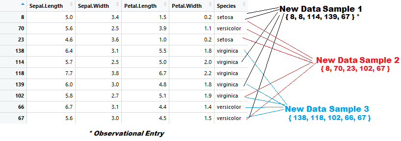
For example, if the following data frame was structured and prepared to serve as a random forest model’s foundation, the first step which would occur during the initial algorithmic process, would be random sampling.

Like the bagging model’s sampling process, the performance of this step might also resemble:

As was previously mentioned, the main differentiating factor which separates the random forest model from the other models whose parts it incorporates, is the manner in which the initial nodal split is designated. In the bagging model, numerous individual trees are created, and each tree is created from the same algorithmic equation as it is applied to each individual data set. In this manner, the optimization pattern is static, while the data for each set is dynamic.

As it pertains to the random forest model, after the creation of each individual set has been established, a pre-selected number of independent variable categories are designated at random from each set, this selection will be assessed by the algorithm, with the most optimal pathway being ultimately selected from amongst the selection of pre-determined variables.

For example, we’ll assume that the number of pre-designate variables which will be selected prior to the creation of each individual tree is 3. If this were the case, each tree within the model will have its initial nodal designation decided upon by which one of the three variables is optimal as it pertains to performing the initial filtering process. The other two variables which are not selected, are then considered for additional nodal splits, along with all of the other variables which the model finds particularly worthy.

With this in mind, a set of variables which would consist of three randomly selected independent variables, might resemble the following as it relates to the initial nodal split:

In this case, the blank node’s logical discretion would be selected from the optimal selection of a single variable from the set: {Sepal.Length, Sepal.Width, Petal.Length}.

One variable would be selected from the set, with the other two variables then being returned to the larger set of all other variables from the initial data frame. From this larger set, all additional nodes would be established based on the optimal placement values determined by the underlying algorithm.

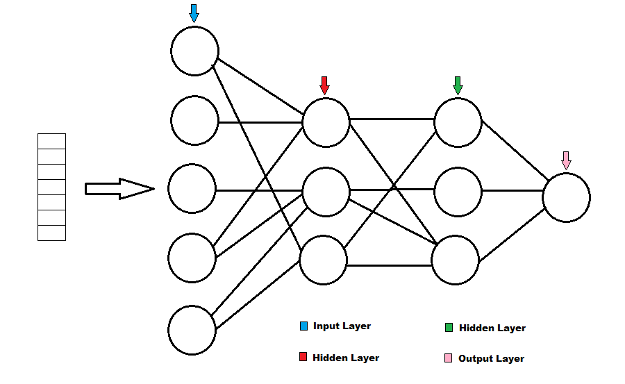
The Decision-Making Process

In a manner which exactly resembles the bagging-boostrap aggregation method described within the prior article, the predictive output figure consists of the majority consensus reached as data is passed through each individual tree model.

The above graphical representation illustrates observation 8 being passed through the model. The model, being comprised of three separate decision trees, which were synthesized from three separate data sets, produces three different internal outcomes. The average of these outcomes is what is eventually returned to the user as the ultimate product of the model.

A Real Application Demonstration (Classification)

Again, we will utilize the "iris" data set which comes embedded within the R data platform.

# Create a training data set from the data frame: "iris" #

# Set randomization seed #

set.seed(454)

# Create a series of random values from a uniform distribution. The number of values being generated will be equal to the number of row observations specified within the data frame. #

rannum <- runif(nrow(iris))

# Order the data frame rows by the values in which the random set is ordered #

raniris <- iris[order(rannum), ]

# With the package "randomForest" downloaded and enabled #

# Create the model #

mod <- randomForest(Species ~., data= raniris[1:100,], type = "class")

# View the model summary #

mod

Console Output:

Call:
randomForest(formula = Species ~ ., data = raniris[1:100, ], type = "class")
Type of random forest: classification
Number of trees: 500
No. of variables tried at each split: 2

               OOB estimate of error rate: 4%
Confusion matrix:
                   setosa versicolor virginica class.error
setosa             31           0            0           0.00000000
versicolor       0          34            1           0.02857143
virginica        0           3           31           0.08823529

Deciphering the Output

Call: - The formula which initially generated the console output.

Type of random forest: Classification – The model type applied to the data frame passed through the “randomForest()” function.

Number of trees: 500 – The number of individual trees from which the data model is comprised of.

No. of variable tried at each split: 2 – The number of randomly selected variables considered as candidates for the initial nodal split criteria.

OOB estimate of error rate: 4% - The amount of erroneous predictions which were discovered within the model as a result of passing OOB (out of bag) data through the completed model.

Class.error – The percentage which appears within the rightmost column represents the total number of observations within the row divided by the number of incorrectly categorized observations within the row.

OOB and the Confusion Matrix

OOB is an abbreviation for “Out of Bag”. As it pertains to the random forest model, as each individual tree is being established within the model, additional observations from the original data set will, as a consequence of the method, not be selected for inclusion as it pertains to the creation the subsets. To generate both the OOB estimate of the error rate, and the confusion matrix within the object summary, the withheld data is passed through each individual tree once it is created. Through an internal tallying and consensus methodology, the confusion matrix presents an estimate of all observational predictions which existed within the initial data set, however, not all of the observational values which were predicted through this method were evenly assessed throughout the entire series of tree models. The consensus is that this test of prediction specificity is superior to testing the complete model with the entire set of initial variables. However, due to the level of complexity which is innate within the methodology, which, as an aspect of such, makes explaining findings to others extremely difficult, I will often also run the standard prediction function as well.

# View model classification results with training data #

prediction <- predict(mod, raniris[1:100,], type="class")

table(raniris[1:100,]$Species, predicted = prediction )

# View model classification results with test data #

prediction <- predict(mod, raniris[101:150,], type="class")

table(raniris[101:150,]$Species, predicted = prediction )

Console Output (1):

predicted
             setosa versicolor virginica
setosa      31      0       0
versicolor 0     35       0
virginica   0      0       34

Console Output (2):

predicted
           setosa versicolor virginica
setosa    19       0            0
versicolor 0     13          2
virginica 0        2          14

As you probably already noticed, the “Console Output (1)” values differ from those produced within the object’s Confusion Matrix. This is a result of the phenomenon which was just previously discussed.

To further illustrate this concept, if I were to change the number of trees to be created to: 2, thus, overriding the package default, the Confusion Matrix will lack enough observations to reflect the total number of observations within the initial set. The result would be the following:

# With the package "randomForest" downloaded and enabled #

# Create the model #

mod <- randomForest(Species ~., data= raniris[1:100,], ntree= 2, type = "class")

# View the model summary #

mod

Call:
randomForest(formula = Species ~ ., data = raniris[1:100, ], ntree = 2, type = "class")
Type of random forest: classification
Number of trees: 2
No. of variables tried at each split: 2

OOB estimate of error rate: 3.57%
Confusion matrix:
          setosa versicolor virginica class.error
setosa        15           0           0      0.00000000
versicolor   0          19           0      0.00000000
virginica     0          2           20      0.09090909

Peculiar Aspects of randomForest

There are few particular aspects of the randomForest package which differ from the previously discussed packages. One of which is how the randomForest() assesses variables within a data frame. Specifically, as it relates to such, the package function requires that variables which will be analyzed must have their types specifically assigned.

To address this, we must first view the data type in which each variable is assigned.

This can be accomplished with the following code:

str(raniris)

Which produces the output:

'data.frame': 150 obs. of 5 variables:
$ Sepal.Length: num 5 5.6 4.6 6.4 5.7 7.7 6 5.8 6.7 5.6 ...
$ Sepal.Width : num 3.4 2.5 3.6 3.1 2.5 3.8 3 2.7 3.1 3 ...
$ Petal.Length: num 1.5 3.9 1 5.5 5 6.7 4.8 5.1 4.4 4.5 ...
$ Petal.Width : num 0.2 1.1 0.2 1.8 2 2.2 1.8 1.9 1.4 1.5 ...
$ Species : Factor w/ 3 levels "setosa","versicolor",..: 1 2 1 3 3 3 3 3 2 2 ...

While this data frame does not require additional modification, if there was a need to change or assign variable types, this can be achieved through the following lines of code:

# Change variable type to continuous #

dataframe$contvar <- as.integer(dataframe$contvar)

# Change variable type to categorical #

dataframe$catvar <- as.factor(dataframe$catvar)

Another unique differentiation which applies to the randomForest() function is the way in which it handles missing observational variable entries. You may recall from when we were previously building tree models within the “rpart” package, that the model methodology included within such contained an internal algorithm which assessed missing variable observational values, and assigned those values “surrogate values” based on other similar variable observations.

Unfortunately, the randomForest() function requires that the user take a on more manual approach as it pertains to working around, and otherwise including these observational values within the eventual model.

First, be sure that all variables within the model are appropriately assigned to the correct corresponding data types.

Next, you will need to impute the data. To achieve this, you will need to utilize the following code for each variable column which is absent data.

# Impute missing variable values #

rfImpute(variablename ~., data=dataframename, iter = 500)

This function instructs the randomForest package library to create new variable entries for whatever the specified variable may be by considering similar entries contained with other variable columns. “iter = “ specifies the number of iterations to utilize when accomplishing this task, as for whatever reason, this method of variable generation requires the creation of numerous tree models. A maximum of 6 iterations is enough to accomplish this task, however, I err on the side of extreme caution. If your data frame is colossal, 6 iterations should suffice.

Though it’s un-necessary, let’s apply this function to each variable within our “iris” data frame:

raniris[1:100,]$Sepal.Length <- rfImpute(Sepal.Length ~., data=raniris[1:100,], iter = 500)

raniris[1:100,]$Sepal.Width <- rfImpute(Sepal.Width ~., data=raniris[1:100,], iter = 500)

raniris[1:100,]$Petal.Length <- rfImpute(Petal.Length ~., data=raniris[1:100,], iter = 500)

raniris[1:100,]$Petal.Width <- rfImpute(Petal.Width ~., data=raniris[1:100,], iter = 500)

raniris[1:100,]$Species <- rfImpute(Species ~., data=raniris[1:100,], iter = 500)

You will receive the error message:

Error in rfImpute.default(m, y, ...) : No NAs found in m

Which correctly indicates that there were no NA values to be found in the initial set.

Variables to Consider for Initial Nodal Split

The randomForest package has embedded within its namesake function, a default assignment as it pertains to the number of variables which are consider for each initial nodal split. This value can be modified by the user for optimal utilization of the model’s capabilities. The functional option to specify this modification is “mtry”.

How would a researcher decide what the optimal value of this option ought to be? Thankfully, a Youtube user named: StatQuest with Josh Starmer, has created the following code to assist us with this decision.

# Optimal mtry assessment #

# vector(length = ) must equal the number of independent variables within the function #

# for(i in 1: ) must have a value which equals the number of independent variables within the function #

oob.values <- vector(length = 4)

for(i in 1:4) {

temp.model <- randomForest(Species ~., data=raniris[1:100,], mtry=i, ntree=1000)

oob.values[i] <- temp.model$err.rate[nrow(temp.model$err.rate), 1]

}

# View the object #

oob.values

Console Output

[1] 0.04 0.04 0.04 0.04

The values produced are the OOB error rates which are associated with each number of variable inclusions.

Therefore, the leftmost value would be the OOB error rate with one variable included within the model. The rightmost value would be the OOB error rate with four variables included with the model.

In the case of our model, as there is no change in OOB error as it pertains to the number of variables utilized for initial nodal split consideration, the option “mtry” can remain unaltered. However, if for whatever reason, we wished to consider a set of 3 random variables for each initial split within our model, we would utilize the following code:

mod <- randomForest(Species ~., data= raniris[1:100,], mtry= 3, type = "class")

Graphing Output

There are numerous ways to graphically represent the inner aspects of a random forest model as its aspects work in tandem to generate a predictive analysis. In this section, we will review two of the simplest methods for generating illustrative output.

The first method creates a general error plot of the model. This can be achieved through the utilization of the following code:

# Plot model #

plot(mod)

# include legend #

layout(matrix(c(1,2),nrow=1),

width=c(4,1))

par(mar=c(5,4,4,0)) #No margin on the right side

plot(mod, log="y")

par(mar=c(5,0,4,2)) #No margin on the left side

plot(c(0,1),type="n", axes=F, xlab="", ylab="")

# “col=” and “fill=” must both be set to one plus the total number of independent variables within the model #

legend("topleft", colnames(mod$err.rate),col=1:4,cex=0.8,fill=1:4)

# Source of Inspiration: https://stackoverflow.com/questions/20328452/legend-for-random-forest-plot-in-r #

This produces the following output: 

This next method creates an output which quantifies the importance of each variable within the model. The type of analysis which determines the variable importance depends on the model type specified within the initial function. In the case of our classification model, the following graphical output is produced from the line of code below:

varImpPlot(mod)

A Real Application Demonstration (ANOVA)

# Create a training data set from the data frame: "iris" #

# Set randomization seed #

set.seed(454)

# Create a series of random values from a uniform distribution. The number of values being generated will be equal to the number of row observations specified within the data frame. #

rannum <- runif(nrow(iris))

# Order the dataframe rows by the values in which the random set is ordered #

raniris <- iris[order(rannum), ]

# With the package "ipred" downloaded and enabled #

# Create the model #

anmod <- randomForest(Sepal.Length ~ Sepal.Width + Petal.Length + Petal.Width, data = raniris[1:100,], method="anova")

Like the previously discussed methodologies, you also have the option of utilizing Root Mean Standard Error, or Mean Absolute Error, to analyze the model’s predictive capacity.

# Compute the Root Mean Standard Error (RMSE) of model training data #

prediction <- predict(anmod, raniris[1:100,], type="class")

# With the package "metrics" downloaded and enabled #

rmse(raniris[1:100,]$Sepal.Length, prediction )

# Compute the Root Mean Standard Error (RMSE) of model testing data #

prediction <- predict(anmod, raniris[101:150,], type="class")

# With the package "metrics" downloaded and enabled #

rmse(raniris[101:150,]$Sepal.Length, prediction )

# Mean Absolute Error #

# Create MAE function #

MAE <- function(actual, predicted) {mean(abs(actual - predicted))}

# Function Source: https://www.youtube.com/watch?v=XLNsl1Da5MA #

# Regenerate Predictive Model #

anprediction <- predict(anmodel , raniris[1:100,])

# Utilize MAE function on model training data #

MAE(raniris[1:100,]$Sepal.Length, anprediction)

# Mean Absolute Error #

anprediction <- predict(anmodel , raniris[101:150,])

# Utilize MAE function on model testing data #

MAE(raniris[101:150,]$Sepal.Length, anprediction)

Console Output (RMSE)

[1] 0.2044091

[1] 0.3709858

Console Output (MAE)

[1] 0.2215909

[1] 0.2632491

Just like the classification variation of the random forest model, graphical outputs can also be created to illustrate the internal aspects of the ANOVA version of the model.

# Plot model #

plot(anmod)

# Measure variable significance #

varImpPlot(anmod)

That's all for this entry, Data Heads.

We'll continue on the topic of machine learning next week.

Until then, stay studious!

-RD

(R) Machine Learning - Bagging, Boosting and Bootstrap Aggregation – Pt. II

Now that you have a fundamental understanding of tree based modeling, we can begin to discuss the concept of "Bootstrap Aggregation". Both of the previously mentioned concepts will come to serve as compositional aspects of a separate model known as "The Random Forest". This methodology will be discussed in the subsequent article.

All three of these concepts classify as "Machine Learning", specifically, supervised machine learning.

"Bagging", is a word play synonym, which serves as a short abbreviation for "Bootstrap Aggregation". Bootstrap aggregation is a term which is utilized to describe a methodology in which multiple randomized observations are drawn from a sample data set. "Boosting" refers to the algorithm which analyzes numerous sample sets which were composed as a result of the previous process. Ultimately, from these sets, numerous decision trees are created. Into which, test data is eventually passed. Each observation within the test data set is analyzed as it passes through the numerous nodes of each individual tree. The results of the predictive output being the consensus of the results reached from a majority of the individual internal models.

How Bagging is Utilized

As previously discussed, "Bagging" is a data sampling methodology. For demonstrative purposes, let's consider its application as it is applied to a randomized version of the "iris" data frame. Here is a portion of the data frame as it currently exists within the "R" platform.

From this data frame, we could utilize the "bagging" methodology to create numerous subsets which contain aspects of the observations contained therein. This methodology will sample from the data frame a pre-determined number of times until it has created a single data sub-set. Once this task has been completed, the process will be completed until a pre-determined number of subsets have been created. Observations from the initial data frame can be sampled multiple times in order to build each individual subset. Therefore, each data frame may contain multiple instances of the same observation.

A graphical representation of this process is illustrated below:

In the case of our illustrated example, three new data samples were created. Each new sample contains a similar number of observations, however, observations from the original data frame are not exclusive in each set. Also, as demonstrated in the above graphic, data observations can repeat within the same sample.

Boosting Described

Once new data samples have been created, the "boosting" process, which is the portion of the algorithm which is initiated following the "bagging" methodology's application, begins to create individualized decision trees for each newly created set. Once each decision tree has been created, the model’s creation process is complete.

The Decision Making Process

With the model created, the process of predicting dependent variable values can be initiated.

Remember that each decision tree was created from data observations from which each corresponding set was comprised of.

The above graphical representation illustrates observation - 8 ,being passed through the model. The model, being comprised of three separate decision trees, which were synthesized from three separate data subsets, produces three different internal outcomes. The average of these outcomes is what is eventually returned to the user as the ultimate product of the model.

A Real Application Demonstration (Classification)

Again, we will utilize the "iris" data set which comes embedded within the R data platform.

A short note on the standard notation utilized for this model type:

D = The training data set.

n = The number of observations within the training data set.

n^1 = "n prime". The number of observations within each data subset.

m = The number of subsets.

In this example we will allow the bagging package command to perform its default function without specifying any additional options. If n^1 = n, then each subset which is created from the training data set is expected to contain at least (1 - 1/e) (≈63.2%) of the unique observations contained within the training data set. If this does not occur, the bagging() function will automatically enable an option which ensures this occurrence.

# Create a training data set from the data frame: "iris" #

# Set randomization seed #

set.seed(454)

# Create a series of random values from a uniform distribution. The number of values being generated will be equal to the number of row observations specified within the data frame. #

rannum <- runif(nrow(iris))

# Order the data frame rows by the values in which the random set is ordered #

raniris <- iris[order(rannum), ]

# With the package "ipred" downloaded and enabled #

# Create the model #

mod <- bagging(Species ~., data= raniris[1:100,], type = "class")

# View model classification results with training data #

prediction <- predict(mod, raniris[1:100,], type="class")

table(raniris[1:100,]$Species, predicted = prediction )

# View model classification results with test data #

prediction <- predict(mod, raniris[101:150,], type="class")

table(raniris[101:150,]$Species, predicted = prediction )

Console Output (1):

predicted

setosa versicolor virginica

setosa 31 0 0

versicolor 0 35 0

virginica 0 0 34

Console Output (2):

predicted

setosa versicolor virginica

setosa 19 0 0

versicolor 0 13 2

virginica 0 2 14

A Real Application Demonstration (ANOVA)

In this second example demonstration, all of the notational aspects of the model and the restrictions of the function still apply. However, in this case, the dependent variable is continuous, not categorical. To test the predictability of the model, the Root Mean Standard Error and the Mean Absolute Error values are calculated. For more information as it pertains to the calculation and interpretation of these measurements of predictability, please consult the prior article.

# Create a training data set from the data frame: "iris" #

# Set randomization seed #

set.seed(454)

# Create a series of random values from a uniform distribution. The number of values being generated will be equal to the number of row observations specified within the data frame. #

rannum <- runif(nrow(iris))

# Order the dataframe rows by the values in which the random set is ordered #

raniris <- iris[order(rannum), ]

# With the package "ipred" downloaded and enabled #

# Create the model #

anmod <- bagging(Sepal.Length ~ Sepal.Width + Petal.Length + Petal.Width, data = raniris[1:100,], method="anova")

# Compute the Root Mean Standard Error (RMSE) of model training data #

prediction <- predict(anmod, raniris[1:100,], type="class")

# With the package "metrics" downloaded and enabled #

rmse(raniris[1:100,]$Sepal.Length, prediction )

# Compute the Root Mean Standard Error (RMSE) of model test data #

prediction <- predict(anmod, raniris[101:150,], type="class")

# With the package "metrics" downloaded and enabled #

rmse(raniris[101:150,]$Sepal.Length, prediction )

Console Output (1) - Training Data:

[1] 0.3032058

Console Output (2) - Test Data:

[1] 0.3427076

# Create a function to calculate Mean Absolute Error #

MAE <- function(actual, predicted) {mean(abs(actual - predicted))}

# Compute the Mean Absolute Error (MAE) of model training data #

anprediction <- predict(anmodel , raniris[1:100,])

MAE(raniris[1:100,]$Sepal.Length, anprediction)

# Compute the Mean Absolute Error (MAE) of model test data #

anprediction <- predict(anmodel , raniris[101:150,])

MAE(raniris[101:150,]$Sepal.Length, anprediction)

Console Output (1) - Training Data:

[1] 0.2289299

Console Output (2) - Test Data:

[1] 0.2706003

Conclusions

The method from which the Bagging() function was derived, was initially postulated by Leo Breiman, the same individual who created the tree model methodology. You will likely never be inclined to use this methodology as a standalone method of analysis. As was previously mentioned within this article, the justification for this topic’s discussion pertains solely its applicability as an aspect of the random forest model. Therefore, from a pragmatic standpoint, if tree models are the model type which you wish to utilize when performing data analysis, you would either be inclined to select the basic tree model for its simplicity, or the random forest model for its enhanced ability.

That's all for today.

I'll see you next week,

-RD