(R) Survival Analysis - Kaplan-Meier and Cox Models (SPSS)

Survival Analysis is a statistical methodology which measures the probability of an event occurring within a group over a period of time.

If you have a decent understanding of the linear regression concept, understanding the output generated by the survival analysis model is fairly simple.

We will demonstrate the methodology of survival analysis through various examples. The data set which will be utilized for the following demonstrations is found within the R “survival” package.

Example: Survival Analysis - Kaplan-Meier Model (R)

# With the R package: “survival” downloaded and enabled #

The R “survival” package comes with the “veteran” data frame embedded within its composition. With the “survival” package enabled, the “veteran” data frame can be called with the command: “veteran”.

If you wish to view this data frame within the R-Studio graphical user interface, you must first assign it to a native data frame variable.

vet1 <- veteran

Double clicking on this data frame variable within the environment frame of R-Studio will present you with the following:

To begin performing a Kaplan-Meier survival analysis within the R platform, you must utilize the following line of code:

kmsurvival <- survfit(Surv(time, status) ~ 1, data=vet1)

This code will indicate to R that a Kaplan-Meier survival analysis should be embarked upon. The “time” variable is indicating the time status, and the “status” variable is indicating censor status (1 = Non-Censored, 0 = Censored). In the case of this particular model, both data frame variables are named exactly what the variable type implies. Please be aware that data frames variables are not always perfectly assigned in this manner.

To view the model output, we will invoke the following function:

summary(kmsurvival)

Which produces the following output:

> summary(kmsurvival)
Call: survfit(formula = Surv(time, status) ~ 1, data = vet1)

time n.risk n.event survival std.err lower 95% CI upper 95% CI
1 137 2 0.985 0.01025 0.96552 1.0000
2 135 1 0.978 0.01250 0.95390 1.0000
3 134 1 0.971 0.01438 0.94302 0.9994
4 133 1 0.964 0.01602 0.93261 0.9954
7 132 3 0.942 0.02003 0.90315 0.9817
8 129 4 0.912 0.02415 0.86628 0.9610
10 125 2 0.898 0.02588 0.84850 0.9500
11 123 1 0.891 0.02668 0.83973 0.9444
12 122 2 0.876 0.02817 0.82241 0.9329
13 120 2 0.861 0.02953 0.80534 0.9212
15 118 2 0.847 0.03078 0.78849 0.9092
16 116 1 0.839 0.03137 0.78013 0.9032
18 115 3 0.818 0.03300 0.75533 0.8848
19 112 2 0.803 0.03399 0.73900 0.8724
20 110 2 0.788 0.03490 0.72280 0.8598

The output itself is much greater in length but I have only included the first 20 observations.

In discussing each unique aspect of the output:

time – This variable illustrates the categorical point in time when a measurement was taken.

n.risk – This variable represents the number of individuals remaining within the initial group of measured individuals.

n.event – This variable represents the total number of individuals who were removed from the remaining group of individuals at the measured point in time.

survival – The probability of any individual within the initial group being a remaining member of the group at this present point in time.

Typically, with survival analysis, the application of the methodology is demonstrated through examples pertaining to drug trials. We could imagine, a scenario which involves patients undergoing treatment for some ailment until their symptoms subside. This gradual diminishment of initial individuals involved in the study is illustrated in the output below:

As the categorical measurement of time progresses (63 – 72), the n.risk figure decreases (72 – 71), this is demonstrated by the number of individuals who no longer meet the initial groups classification (n.event = 1). However, how can we explain the phenomenon in which more individuals leave the study than are not accounted for? This is the case for the numerical values encircled in blue.

You may recall earlier, that we specified for the variable “status” within our “survfit” function. What does this variable connotate within the context of our original data frame?

Censoring

As it pertains to survival analysis, the term “censoring” refers to the event in which an individual leaves the original group without the measured even occurring. For example, in the case of a study, this could occur if an individual stops corresponding with the researchers. Or for a more morbid example, if an individual passes away as a result of circumstance un-related to the study.

In either situation, this non-event loss of individuals from the initial group will be connotated by a cross marking on the graphed output. These individuals are considered “censored” individuals.

To create a graphical output for our example model, we would utilize the following code:

# With the R packages: “ggplot2”, and "ggfortify" downloaded and enabled #

autoplot(kmsurvival)

Which produces the following output:

The center solid line represents the survival probability of the model, the outside grey area represents the 5% and 95% confidence intervals. The cross markings on the solid central line indicate an instance when censoring took place.

Example: Survival Analysis - Kaplan-Meier Model (R)

We will now produce a model which contains the same parameters of the previous model. The graphical output created as a result of such is the product of two separate sets of analysis, each set specifying a pre-determined condition. Each conditional scenario will be illustrated within the model output as separate solid lines.

To achieve this desired results, we must run the following lines of code:

# With the R package: “survival” downloaded and enabled #

# In this case, our factor is “trt” #

kmsurvival <- survfit(Surv(time, status) ~ trt, data=vet1)

To view the model output, we will invoke the following function:

summary(kmsurvival)

Which produces the following output:

Call: survfit(formula = Surv(time, status) ~ trt, data = vet1)
trt=1
time n.risk n.event survival std.err lower 95% CI upper 95% CI
3 69 1 0.9855 0.0144 0.95771 1.000
4 68 1 0.9710 0.0202 0.93223 1.000
7 67 1 0.9565 0.0246 0.90959 1.000
8 66 2 0.9275 0.0312 0.86834 0.991
10 64 2 0.8986 0.0363 0.83006 0.973
11 62 1 0.8841 0.0385 0.81165 0.963
12 61 2 0.8551 0.0424 0.77592 0.942
13 59 1 0.8406 0.0441 0.75849 0.932
16 58 1 0.8261 0.0456 0.74132 0.921
18 57 2 0.7971 0.0484 0.70764 0.898
20 55 1 0.7826 0.0497 0.69109 0.886

(and)

trt=2
time n.risk n.event survival std.err lower 95% CI upper 95% CI
1 68 2 0.9706 0.0205 0.93125 1.000
2 66 1 0.9559 0.0249 0.90830 1.000
7 65 2 0.9265 0.0317 0.86647 0.991
8 63 2 0.8971 0.0369 0.82766 0.972
13 61 1 0.8824 0.0391 0.80900 0.962
15 60 2 0.8529 0.0429 0.77278 0.941
18 58 1 0.8382 0.0447 0.75513 0.930
19 57 2 0.8088 0.0477 0.72056 0.908
20 55 1 0.7941 0.0490 0.70360 0.896

Again, I shortened the output to conserve space. However, as is evident within the portions of output, each particular condition is illustrated above the conditional output type. (trt = 1, trt = 2)

To create a graphical output for our example model, we would utilize the following code:

# With the R packages: “ggplot2”, and "ggfortify" downloaded and enabled # 

autoplot(kmsurvival)

Which produces the following output:

Notice that in this case, two separate confidence interval areas have been produced, each pair existing as an aspect of the solid line in which it engulfs.

Example: Survival Analysis – Cox Proportional Hazard Model (R)

The Cox Proportional Hazard Model, like the Kaplan-Meier Model, is also a survival analysis methodology. The Cox Model is more complicated in its composition as it allows for the inclusion of additional variables. The inclusion of these additional variables, if correctly integrated, can yield a more descriptive model. However, as a consequence of the model’s complication, the additional aspects which provide positive differentiation, can also lead to the increased probability of user error.

To create a Cox Proportional Hazard Model, we will utilize the following lines of code:

# With the R package: “survival” downloaded and enabled #

coxsurvival <- coxph(Surv(time, status) ~ trt + karno + diagtime + age + prior , data=vet1)

summary(coxsurvival)

This produces the output:

Call:
coxph(formula = Surv(time, status) ~ trt + karno + diagtime +
age + prior, data = vet1)

n= 137, number of events= 128

coef exp(coef) se(coef) z Pr(>|z|)
trt 0.193053 1.212947 0.186446 1.035 0.300
karno -0.034084 0.966490 0.005341 -6.381 1.76e-10 ***
diagtime 0.001723 1.001725 0.009003 0.191 0.848
age -0.003883 0.996125 0.009247 -0.420 0.675
prior -0.007764 0.992266 0.022152 -0.350 0.726
---
Signif. codes: 0 ‘***’ 0.001 ‘**’ 0.01 ‘*’ 0.05 ‘.’ 0.1 ‘ ’ 1

exp(coef) exp(-coef) lower .95 upper .95
trt 1.2129 0.8244 0.8417 1.7480
karno 0.9665 1.0347 0.9564 0.9767
diagtime 1.0017 0.9983 0.9842 1.0196
age 0.9961 1.0039 0.9782 1.0143
prior 0.9923 1.0078 0.9501 1.0363

Concordance= 0.714 (se = 0.03 )
Rsquare= 0.271 (max possible= 0.999 )
Likelihood ratio test= 43.27 on 5 df, p=3.259e-08
Wald test = 44.88 on 5 df, p=1.537e-08
Score (logrank) test = 47.39 on 5 df, p=4.734e-09

Primarily, when analyzing the model summary data, we should concern ourselves with the portions of the output which I have highlighted in bold. The initial portion of the output provides values, which are found within the rightmost column, which indicate the strength of each variable as it impacts the overall outcome of the model (Pr(>|z|).

The p-value of the Wald Test (1.537e-08 < .05), indicates that the model is significant. While the r-squared value (.271), indicates that the model is not a particularly good fit as it pertains to the existing data points.

To create a graphical output for our example model, we would utilize the following code:

# With the R packages: “ggplot2”, and "ggfortify" downloaded and enabled # 

coxsurvival <- survfit(coxsurvival)

autoplot(coxsurvival)

Which produces the following output:

Example: Survival Analysis – Cox Proportional Hazard Model with Time Dependent Co-Variates (R) 

There may be instances in which you will encounter survival data which contains time dependent co-variates. What this translates to, in simpler terms, is that the data which you are preparing to analyze contains variables which are dependent on time duration.

The data in these scenarios is typically organized in a manner similar to data presented below:

As is demonstrated within the data set, individuals have been surveyed multiple times. This method has been utilized to account for the variables “symphtomA” and “symphtomB”, which typically occur as a result of the treatment methods occurring over set intervals of time.

It may appear that the time intervals are overlapping in the above example, however, this is not the case. When setting up data for analysis in the manner, it must be structured similarly, with duration aspects appearing to overlap. The lack of ambivalence is due to measurements being taken at the end of each interval. So, in the case of ID:3, measurements were taken at day 50, day 100, day 150, day 200, and day 250.

To begin performing a Cox Proportional Hazard Model with Time Dependent Co-Variates within the R platform, you must utilize the following lines of code:

(I am aware that this sample data, model, and graphical output are equally awful. However, I could not find a worthwhile example to demonstrate, and making data sets from scratch which contain decent representational entries is extremely difficult. The .csv file utilized to create this example can be found at the end of the article.)

coxsurvival1 <- coxph(Surv(time1, time2, status) ~ trt + karno + diagtime + age + symphtomA + symphtomB , data=vet2)

summary(coxsurvival1)

This produces the output:

Call:
coxph(formula = Surv(time1, time2, status) ~ trt + karno + diagtime +
age + symphtomA + symphtomB, data = vet2)

n= 22, number of events= 21

coef exp(coef) se(coef) z Pr(>|z|)
trt 3.959e-16 1.000e+00 1.225e+00 0.000 1.000
karno -2.636e-17 1.000e+00 8.672e-02 0.000 1.000
diagtime -1.281e-16 1.000e+00 1.713e-01 0.000 1.000
age 2.730e-17 1.000e+00 5.009e-02 0.000 1.000
symphtomA -9.177e-16 1.000e+00 7.906e-01 0.000 1.000
symphtomB -1.985e+01 2.392e-09 1.510e+04 -0.001 0.999

exp(coef) exp(-coef) lower .95 upper .95
trt 1.000e+00 1.00e+00 0.09061 11.036
karno 1.000e+00 1.00e+00 0.84370 1.185
diagtime 1.000e+00 1.00e+00 0.71474 1.399
age 1.000e+00 1.00e+00 0.90649 1.103
symphtomA 1.000e+00 1.00e+00 0.21236 4.709
symphtomB 2.392e-09 4.18e+08 0.00000 Inf

Concordance= 1 (se = 1.594 )
Rsquare= 0.118 (max possible= 0.723 )
Likelihood ratio test= 2.77 on 6 df, p=0.8368
Wald test = 0 on 6 df, p=1
Score (logrank) test = 1.78 on 6 df, p=0.9389

To create a graphical output for our example model, we would utilize the following code:

# With the R package: “survival” downloaded and enabled #

coxsurvival1 <- survfit(coxsurvival1)

autoplot(coxsurvival1)

Which produces the following output:

Example: Survival Analysis - Kaplan-Meier Model (SPSS)

To re-create this example, you must first export the “veteran” data set to a .csv file, and then subsequently import it into the SPSS platform.

The result of such should resemble the following:

To begin, you must first select “Analyze” from the upper left drop down menu, then select “Survival”, followed by “Kaplan-Meier”.

This should present the following interface:

Utilizing the top center arrow, designate the variable “time” as the “Time” entry. Then, utilize the second topmost arrow to designate the variable “status” as the “Status” entry.

Once this step has been completed, click on the box labeled “Define Event”.

From the sub-menu generated, input “1” as the “Single value”, then click “Continue”.

Next, click on the menu box labeled “Options”.

This should cause the following menu to populate:

Be sure to check the boxes to the left of the “Mean and medial survival” and “Survival” options.

Once this is completed, click “Continue”, and then click “OK”.

This s will generate the following output:

The model parameters can be modified in the initial menu to produce an output which is differentiated by a factor variable.

This modification would produce the output:

Example: Survival Analysis – Cox Proportional Hazard Model (SPSS)

We will be utilizing the same data set which analyzed in the previous example:

To begin, you must first select “Analyze” from the upper left drop down menu, then select “Survival”, followed by “Cox Regression”.

This should present the following interface:

Utilizing the top center arrow, designate the variable “time” as the “Time” entry. Then, utilize the second topmost arrow to designate the variable “status” as the “status” entry. Finally, utilize the middle center arrow to designate the variables “trt”, “karno”, “diagtime”, “age”, and “prior” as “Covariates”.

Once this step has been completed, click on the box labeled “Define Event”.

From the sub-menu generated, input “1” as the “Single value”, then click “Continue”.

Next, click on the menu option labeled “Plots”.

Within this interface, select the box to the left of the option labeled “Survival”, then click “Continue”.

Once this has been completed click “OK”.

This should produce the following output:

Survival Analysis – Cox Proportional Hazard Model Example File (.csv)

id,trt,celltype,time1,time2,status,karno,diagtime,age,prior,symphtomA,symphtomB
1,1,squamous,0,50,1,60,7,69,0,0,0
1,1,squamous,50,100,1,60,7,69,0,1,0
2,1,squamous,0,50,1,70,5,64,10,1,0
2,1,squamous,50,100,1,70,5,64,10,0,0
2,1,squamous,100,150,1,70,5,64,10,1,0
2,1,squamous,150,200,1,70,5,64,10,1,0
2,1,squamous,200,250,1,70,5,64,10,1,0
2,1,squamous,250,300,1,70,5,64,10,1,0
2,1,squamous,300,350,1,70,5,64,10,1,1
2,1,squamous,350,400,1,70,5,64,10,1,1
2,1,squamous,400,450,1,70,5,64,10,1,1
3,2,squamous,0,50,1,60,3,38,0,0,0
3,2,squamous,50,100,1,60,3,38,0,1,0
3,2,squamous,100,150,1,60,3,38,0,1,0
3,2,squamous,150,200,1,60,3,38,0,1,0
3,2,squamous,200,250,1,60,3,38,0,1,0
4,2,squamous,0,50,1,60,9,63,10,0,0
4,2,squamous,50,100,1,60,9,63,10,1,0
4,2,squamous,100,150,1,60,9,63,10,1,0
5,1,squamous,0,50,1,70,11,65,10,0,0
5,1,squamous,50,100,1,70,11,65,10,0,0
5,1,squamous,100,150,0,70,11,65,10,0,1

That’s all for now, Data Heads! Stay tuned for more informative content!

(R) Odds Ratio, Relative Risk and Cohen’s Kappa

In this article, we will be discussing Odds Ratio, Relative Risk, The Cohen's Kappa Statistic, and their relation to data contained within contingency tables. Additionally, I will be sharing some code which I have created within the R platform which will simplify the process of generating these figures.

Example:

We will address the typical scenario which involves smoking as it relates to cancer diagnosis.

We will create three data vectors. Each data vector will contain data collected from a single individual. The first data vector will contain an identification variable pertaining to individual. The next data vector will contain a binary variable which identifies smokers and non-smokers alike. The final variable will indicate which individuals are afflicted with cancer.

# Create Data Vectors #

id <- c(1,2,3,4,5,6,7,8,9,10,11,12,13,14,15,16,17,18,19,20)

smoker <- c(0,0,0,1,1,0,0,1,1,1,1,1,0,1,1,1,0,0,0,0)

cancer <- c(0,0,1,1,0,0,1,1,1,1,1,1,0,0,1,1,1,0,0,0)

smokerscancer <- data.frame(id, smoker, cancer)

This data frame now must be transformed into a matrix before it can be analyzed.

This can be achieved through the following code:

# Organize Data into Contingency Table #

x <- smokerscancer$smoker

y <- smokerscancer$cancer

cases <- data.frame(x,y)

cases$y <- c(ifelse(cases$y == 1, 'aTrue', 'bFalse'))

cases$x <- c(ifelse(cases$x == 1, 'aTrue', 'bFalse'))

cases <- cases[complete.cases(cases), ]

ctable <- table(cases)

# Apply Chi-Squared Test of Independence #

chisq.test(ctable)

Which produces the following output:

Pearson's Chi-squared test with Yates' continuity correction

data: ctable
X-squared = 3.2323, df = 1, p-value = 0.0722

For more information as how to interpret Chi-squared output, please consult this article.

The following code produces additional output, along with the original contingency table:

# Produce Odds Ratio / Relative Risk Outputs #

totala <- ctable[1,1] + ctable[1,2]
totalb <- ctable[2,1] + ctable[2,2]
percent1 <- (ctable[1,1] / totala) * 100
percent2 <- (ctable[1,2] / totala) * 100
percent3 <- (ctable[2,1] / totalb) * 100
percent4 <- (ctable[2,2] / totalb) * 100
totalc <- ctable[1,2] + ctable[2,2]
totald <- ctable[1,1] + ctable[2,1]
totale <- totalc + totald
rowtotala <-totald/(totalc + totald) * 100
rowtotalb <-totalc/(totalc + totald) * 100
rowtotalc <- (rowtotala + rowtotalb)

keycol <- c("Count", "(%)", "Count", "(%)", "SumCount", "(%)")
col1 <- c(ctable[1,1], percent1, ctable[2,1], percent3, totald, rowtotala)
col2 <- c(ctable[1,2], percent2, ctable[2,2], percent4, totalc, rowtotalb)
rowtotals <- c((ctable[1,1] + ctable[1,2]), (percent1 + percent2), (ctable[2,1] + ctable[2,2]), (percent3 + percent4), (totalc + totald), rowtotalc)

data <- data.frame(keycol, col1, col2, rowtotals)

vala <- percent3 / percent1
valb <- percent4 / percent2
valab <- valb/vala

num <- (ctable[1,1]) / (ctable[1,1] + ctable[1,2])
den <- (ctable[2,1]) / (ctable[2,1] + ctable[2,2])
relrisk <- num/den

ctable

data

valab # (Odds Ratio) col1 (%/%) / col2 (%/%) #

relrisk # Relative Risk = TRUE col1 (%/%) #

Which produces the following output:

        y
x           aTrue bFalse
aTrue       8        2
bFals      3        7

       keycol    col1    col2    rowtotals
1      Count     8        2          10
2      (%)       80      20       100
3      Count    3        7         10
4      (%)     30      70        100
5      SumCount 11 9         20
6     (%)     55      45 1      00

valab # (Odds Ratio) col1 (%/%) / col2 (%/%) #

[1] 9.333333

relrisk # Relative Risk = TRUE col1 (%/%) #

[1] 2.666667

This output was created to resemble the table generated by SPSS as it pertains to chi-squared contingency data.

But how are the results within this table interpreted?

If your data is structured in the manner in which the contingency table within the example is organized, we can make the following statements.

Risk ratios indicated that the risk of the outcome variable (cancer), within the category of smokers, increased by 167 %* relative to the group of non-smokers. Or, the outcome of this event was 2.667 times more likely to occur within the smoker group.

The odds ratio indicates that the odds of finding cancer within an individual who smokes, as compared to an individual who does not smoke, is 9.333.

*= Absolute value of (1 – RR), multiplied by 100.

Cohen’s Kappa

Cohen’s Kappa, like the odds ratio and the risk ratio, is utilized to analyze the relationships of data within a contingency table. However, while the previously mentioned methods are universally applicable, Cohen’s Kappa can only be applied to contingency tables which measure categorical ratings.

Example:

Two film critics are rating a series of 20 movies. Each critic can either vote “Yes”, as an indication that he enjoyed the film, or “No”, as an indication that he did not enjoy the film. The results were recorded within a binary format.

# Create Vectors #

movieid <- c(1,2,3,4,5,6,7,8,9,10,11,12,13,14,15,16,17,18,19,20)

criticoneratings <- c(0,0,0,1,1,0,0,1,1,1,1,1,0,1,1,1,0,0,0,0)

critictworatings <- c(0,0,1,1,0,0,1,1,1,1,1,1,0,0,1,1,1,0,0,0)

movieratings <- data.frame(movieid, criticoneratings, critictworatings)

With this information, we wish to measure the level of agreement between the two raters. One of the main ways in which this technique differs from traditional probabilistic methodologies, is that this particular technique accounts for chance agreement.

Now that we have our data values correctly input, we can proceed with the analysis.

# Organize Data into Contingency Table #

x <- movieratings$criticoneratings

y <- movieratings$critictworatings

cases <- data.frame(x,y)

cases$y <- c(ifelse(cases$y == 1, 'aTrue', 'bFalse'))

cases$x <- c(ifelse(cases$x == 1, 'aTrue', 'bFalse'))

cases <- cases[complete.cases(cases), ]

ctable <- table(cases)

# With the “psych” package downloaded and enabled #

cohen.kappa(ctable,alpha=.05)

This produces the output:

Call: cohen.kappa1(x = x, w = w, n.obs = n.obs, alpha = alpha, levels = levels)

Cohen Kappa and Weighted Kappa correlation coefficients and confidence boundaries
             lower estimate upper
unweighted kappa    0.12      0.5    0.88
weighted kappa        0.12      0.5    0.88

Number of subjects = 20

I have bolded the kappa statistic (.5) contained within the output.

Opinion as to how to interpret the kappa statistic varies. Written below are the recorded opinions of professional analysts pertaining to such:

“Landis and Koch, characterized values < 0 as indicating no agreement, and 0-0.20 as slight, 0.21-0.40 as fair, 0.41-0.60 as moderate, 0.61-0.80 as substantial, and 0.81-1 as almost perfect agreement.

Fleiss's equally arbitrary guidelines characterize kappa over 0.75 as excellent, 0.40 to 0.75 as fair to good, and below 0.40 as poor. “ **

**- https://en.wikipedia.org/wiki/Cohen’s_kappa

If we were to apply this model in more gregarious manner, for the sake of spectating at the aspects of its inner workings, the following code could be applied:

# Observed Proportionate Agreement #

# Define Cell Entries #

a <- ctable[1,1]
b <- ctable[1,2]

c <- ctable[2,1]
d <- ctable[2,2]

# Observed Proportionate Agreement (p0) #

p0 <- (a + d) / (a + b + c + d)

# Expected probability that both would say yes at random (pYes) #

pyes <- ((a + b) / (a + b + c + d)) * ((a + c) / (a + b + c + d))

# Expected probability that both would say no at random (pNo) #

pno <- ((c + d) / (a + b + c + d)) * ((b + d) / (a + b + c + d))

# Overall random agreement probability is the probability that they #
# agreed on either Yes or No (pe) #

pe <- pyes + pno

# Cohen's Kappa #

K <- (p0 - pe) / (1 - pe)

That’s all for now, Data Heads! Stay tuned for more awesome articles!

(R) Repeated Measures Logistic Regression

One of the more eclectic and synthetic methods of model creation, combines the logistic regression model, with the ability to attribute for multiple re-occurring observations. I heavily advise against utilizing this method for three reasons. The first reason being, is that it is incredibly complicated. The second reason being, is that the math involved is synthetic and combines multiple concepts into a single model methodology. The final reason, is that the code utilized to aid in the model's creation, only exists within an auxillary R package, and the package itself is difficult to utilize.

However, for the sake of demonstration, here is what the code for this method might resemble:

Example:

# Create data vectors #

id <- c(1,1,1,1,1,1,2,2,2,2,2,2,3,3,3,3,3,3)

vara <- c(0,0,0,0,1,1,1,1,1,0,1,1,0,1,1,1,1,0)

varb <- c(0,0,0,0,0,0,1,1,1,0,0,1,1,1,1,0,0,0)

outcome <- c(1,1,1,1,0,0,1,1,1,1,1,0,0,0,0,0,1,1)

# With the package: “lme4”, installed and enabled #

# Apply The Repeated Measures Logistic Regression Model #

glmer(outcome~vara+varb +(1|id),family=binomial)

This creates the output:

Generalized linear mixed model fit by maximum likelihood (Laplace Approximation) ['glmerMod']
Family: binomial ( logit )
Formula: outcome ~ vara + varb + (1 | id)
    AIC BIC logLik deviance df.resid
26.5032 30.0647 -9.2516 18.5032 14
Random effects:
Groups Name          Std.Dev.
id      (Intercept)       2.592
Number of obs: 18, groups: id, 3
Fixed Effects:
(Intercept)            vara           varb
        4.656          -3.757        -3.587

Which can be utilized to create a model equation.

For our example, we can assume that we have three individuals who are being tested for a binary outcome. The variables, which we believe will be impactful within this situation, are the independent variables: “vara” and “varb”. As each individual was surveyed multiple times, the repeated measures logistic regression model was utilized to attribute for this aspect of the experimental methodology.

That’s all for now data heads. Stay tuned for more useful content!

Frequency and Syntax (SPSS)

There are not many articles or videos online which specifically address the topic of “syntax”. Syntax, in this particular instance, refers to the coding language of IBM SPSS. In this article, I will briefly discuss a few useful elements which should lead to an increase in coding efficiency and a greater understanding of IBM SPSS coding syntax. Examples will primarily focus on situations which require the utilization of frequency analysis.

Creating New Syntax

To create new syntax, you must first select “File” from the upper left drop down menu, then select “New”, followed by “Syntax”.

Thus should present the following interface:

The right section of the screen serves as the console. It is this section where you will be creating your code.

I typically begin my code files with the following lines:

* Encoding: UTF-8.

* Establish working directory

cd 'C:\DirectoryPathWay\User\etc\'.

* Specify file path (make sure extension is included)

GET FILE='ExampleFile.sav'.

The first line:

cd 'C:\DirectoryPathWay\User\etc\'.

Establishes the directory from which you will be accessing your files.

The next line:

GET FILE='ExampleFile.sav'.

Is specifying the file in which the code will be referring to when performing specific functions.

You will, of course, have to modify both of the lines above so that they refer to non-fictitious items.

To run syntax from the console, you must first highlight the portions in which you wish to run, then click on the green arrow above.

If the code was correctly formatted and did not produce any errors, the output created as a product of the code’s utilization will be displayed within the output window.

The best way to generate examples of code to provide functions which you wish to utilize, is to first initiate a function from the graphical user interface. Doing such, provides the product of the function to be displayed within the output window. Along with such, is the code, which if ran as syntax, would also perform the same function.

Example (SPSS):

Let us consider the following data set:

With data labels assigned and enabled, the set resembles the following:

To perform a basic frequency analysis output, we must make the following selections. From the topmost menu bar, select “Analyze”, then select “Descriptive Statistics”, finally, select “Frequencies”.

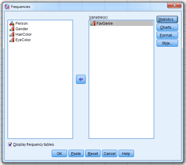
This should cause the following menu to appear:

Utilizing the center arrow, we will designate the column “FavGenre” as our “Variable(s)”.

Once this step has been completed, click “OK”.

The following output will be produced:

Let us turn out attention to the text above the title “Frequencies”.

This output illustrates the code which was utilized as a function to generate the requested analytical output.

This code can be copied and re-utilized from the console window to re-create the output. This can be helpful when multiple queries are required, as it eliminates the tedious process of utilizing the user interface for each independent request.

For example, if you wanted to run the frequency function for multiple variables independently, you could utilize the following code:

Something that I would recommend, and this is completely optional, is the utilization of titles within your code. I find that titles being included within the output, especially when multiple functions are utilized, allows for increased readability and enhanced organization of results.

The inclusion of such would resemble:

Which would produce an output resembling:

For frequencies, if you wished to produce multiple outputs for different variables but did not want create each function independently, you could utilize the following code:

SPSS also provides a function that can be utilized to produce descriptive statistics.

To perform a descriptive frequency output, we must make the following selections. From the topmost menu bar, select “Analyze”, then select “Descriptive Statistics”, finally, select “Descriptive”.

From the menu that is generated from this series of actions, utilize the middle arrow to designate the column “FavGenre” as a “Variable(s)”.

From the sub-menu generated from selecting the “Options” box, make the following selections:

Once this has been completed, click “Continue”, and then click “OK”.

This will produce the following output:

Though it is inapplicable as it pertains to our current example, if there is a situation in which you wish to generate descriptive summary output, the following syntax can be utilized:

DESCRIPTIVES VARIABLES=Height
/STATISTICS=MEAN STDDEV MIN MAX.
If you would like to perform this function from the graphical interface, please follow the proceeding steps. From the topmost menu bar, select “Analyze”, then select “Descriptive Statistics”, finally, select “Descriptives”.



After designating the appropriate variable for analysis. A table similar to the output below should be produced.

Generating these sorts of summaries is rather simple and straightforward. However, what if we wanted to analyze data based on specific criteria?

For our example, we will assume that we only want to generate a frequency table which lists the preferred music genre for females.

The code to achieve such is as follows:

The filter temporarily disables data observations which contain a variable which matches the specified value.

If you were to run this code block independently, you would notice the following impact which it has on the data frame.

The initial lines of code perform the query itself, with the final line disabling the filter. It is important that the filter be disabled (FILTER OFF.), if additional queries are to be performed which do not specifically pertain to the parameters of the current analysis.

WARNING!!!

If you are presented with errors when applying filters, these prompts will typically stem from one of the following:

1. You are applying a filter to a data label. Remember in cases which require such filtering, to always apply the filter to the underlying numerical variable.

2. If you are applying a filter to a string variable, do not forget to include the variable within quotes (‘ ‘) .

If there is a situation in which you must apply multiple filters prior to performing analysis, the following code blocks should provide useful:

Applying multiple filters:

USE ALL.

COMPUTE filter_$=(Gender=0 AND Gender=1).

FILTER BY filter_$.

EXECUTE.

Setting a query variable to NOT EQUAL a value:

USE ALL.

COMPUTE filter_$=(Gender NE 0).

FILTER BY filter_$.

EXECUTE.

Generating query data where a variable equals one value OR another value:

USE ALL.

COMPUTE filter_$=(FavGenre = 1 OR FavGenre = 2).

FILTER BY filter_$.

EXECUTE.

That’s all for now, Data Heads! Stay subscribed for more informative content!

2-Stage Least Squares Regression (SPSS)

Often used in Econometrics, The 2-Stage Least Squares Regression method is a technique which is utilized to create a predictive model which is influenced by, but does not contain, outside variables. These “outside variables” are better known by their proper term, “instrumental variables”.

The definition of an “instrumental variable” is as follows:

“A variable used to estimate casual relationships when controlled experiments are not feasible, or when a treatment is not successfully delivered to every unit in a randomized experiment.” *

In simplified terms, what this essentially means, is that a variable is factored into the regression model which impacts the dependent variables, and as a consequence of such, also impacts the independent variable. Within the model, there can be more instrumental variables than independent variables. However, there cannot be more independent variables than instrumental variables.

Assembling this model manually is rather difficult when synthesizing it by hand. Thankfully, modern technology has granted us the ability to easily create the model within SPSS.

Example (SPSS):

Below is our sample data set:

To begin our analysis, we must select, from the topmost menu, “Analyze”, then “Regression”, followed by “2-Stage Least Squares”.

This sequence of actions should cause the following menu to appear:

Using the topmost arrow button, assign “Z” as a ”Dependent” variable. Once this has been completed, utilize the center arrow button to assign the variables (“Y”, “X”) as “Factor(s)”. Finally, utilize the bottom center arrow button to designate the variables (“Y”, “X”) as “Instrumental” variables.

Next, click on the button labeled “Options”, this should populate the following menu:

From this interface, beneath the header labeled, “Save New Variables”, select the following option: “Predicted”.

Once this has been completed, click the box labeled “Continued”, then select the box labeled “OK”.

This should produce the following output:

The output indicates that the model generated through the utilization of the 2-Stage Least Squares Regression is of extremely poor quality. This is illustrated in the R-Square value (.001), the significance values of the predictor variables (.923, .952, .953), and extremely high correlation value (-.996).

Assuming that the model did serve as a decent predictor, and therefore as such, you desired to use it as a predictive tool, the equation to generate dependent variable values would be as follows:

Dependent Variable Value = (X * 8.369) + (Y * -4.555) + 507.242

SPSS computes the predicted values of the dependent variables from the application of the model as it pertains to the original data set. This is a result of the “Save” option being selected earlier. These predicted values are output into a column within the original data set.

*- https://en.wikipedia.org/wiki/Instrumental_variables_estimation

(R) Probit Regression (SPSS)

Providing the same function of the Logistic Regression Model, and structured in a similar manner, The Probit Regression model provides an alternative to The Logistic Regression Model if the practitioner wishes to pursue a differing methodology.

The only difference in synthesis of the two models, and this aspect of differentiation is minor at best, is the size of the tails which are inherent in the each model’s creation. The Logit model produces slightly flatter tails. This is the sole unique aspect which separates the two models when utilized within an applied setting.

For this reason, due to the wider adoption of the logistic regression model, I would recommend against utilizing the Probit Regression methodology unless explicitly instructed to do so otherwise.

Example (SPSS):

This is where the probit methodology would be demonstrated within the SPSS platform. However, I cannot seem to discern from the interface, or the internet, as to how this would be achieved.

It would seem that I am not alone in my confusion:

http://www-01.ibm.com/support/docview.wss?uid=swg21480469

Example (R):

I will now briefly explain how to create the model within the R platform.

# Create data vectors #

age <- c(55.00, 45.00, 33.00, 22.00, 34.00, 56.00, 78.00, 47.00, 38.00, 68.00, 49.00, 34.00, 28.00, 61.00, 26.00)

obese <- c(1.00, .00, .00, .00, 1.00, 1.00, .00, 1.00, 1.00, .00, 1.00, 1.00, .00, 1.00, .00)

smoking <- c(1.00, .00, .00, 1.00, 1.00, 1.00, .00, .00, 1.00, .00, .00, 1.00, .00, 1.00, 1.00)

cancer <- c(1.00, .00, .00, 1.00, .00, 1.00, .00, .00, 1.00, 1.00, .00, 1.00, 1.00, 1.00, .00)

# Combine data vectors into a single data frame #

cancerdata <- data.frame(cancer, smoking, obese, age)

# Create Probit Model #

probitmodel <- glm(cancer ~ smoking + obese + age, family=binomial(link= "probit"), data=cancerdata)

# Generate Model Summary #

summary(probitmodel)

This produces the output:

Call:

glm(formula = cancer ~ smoking + obese + age, family = binomial(link = "probit"),
data = cancerdata)

Deviance Residuals:
Min       1Q         Median 3Q       Max
-1.6239 -0.7546 0.5868 0.8184 1.8403

Coefficients:

            Estimate        Std. Error z value Pr(>|z|)
(Intercept) -1.40234 1.30773 -1.072 0.284
smoking     1.55682 0.88940 1.750 0.080 .
obese         -0.24549 0.82711 -0.297 0.767
age              0.01792 0.02413 0.743 0.458
---
Signif. codes: 0 ‘***’ 0.001 ‘**’ 0.01 ‘*’ 0.05 ‘.’ 0.1 ‘ ’ 1

(Dispersion parameter for binomial family taken to be 1)

Null deviance: 20.728 on 14 degrees of freedom
Residual deviance: 16.795 on 11 degrees of freedom
AIC: 24.795

Number of Fisher Scoring iterations: 4

Which enables for the creation of the model equation:

Logit(p) = -1.40234 + (Smoking * 1.55682) + (Obese * -0.23549) + (Age * 0.01792)

Which can be implemented within the R platform as:

# Smoking #

Smoking <- 0

# Obese #

Obese <- 0

# Age #

Age <- 0

p <- -1.40234 + (Smoking * 1.55682) + (Obese * -0.23549) + (Age * 0.01792)

plogis(p)

The output of such will provide the probability of the occurrence of the dependent binary variable.

To check for model fit, we will utilize the Nagelkerke R-Squared statistic.

# Generate Nagelkerke R Squared #

# Download and Enable Package: "BaylorEdPsych" #

PseudoR2(probitmodel)

This series of actions presents the following output:

McFadden         Adj.McFadden          Cox.Snell        Nagelkerke
0.1897432            -0.2927030             0.2306398        0.3079774

McKelvey.Zavoina           Effron
0.3228210                     0.2436036

Count           Adj.Count          AIC                Corrected.AIC
0.7333333      0.4285714      24.7947590         28.7947590

The only value which we need to concern ourselves with is the Nagelkerke value. As this value is interpreted in way which is similar to that of the typical R-Squared value, at .308, we can determine that this model is not a good fit for the data.

There are additional aspects of interpretation that can be discerned from this model, and these interpretations are similarly applicable as they pertain to the logistic regression model. For more information as to how these methods of interpretation are utilized, please consult the entry titled: Logistic Regression Analysis (Binary Categorical Variables).

(R) Logistic Ordinal Regression (SPSS)

As if multinomial logistic regression was not confusing enough, today, we will be discussing an even more vexing variation of the logistic regression model. The model which will the topic of this article is: Logistic Ordinal Regression.

The Logistic Ordinal Regression Model is incredibly similar in concept as compared to the multinomial logistic regression model. Both models are utilized to assess ordinal variable outcomes through logistical methodologies. The primary differentiation between the two models pertains to model synthesis and output. If you have an intimate understandings of these differences, selecting the appropriate model should be a relatively simple task. However, if you do not have significant insight as to what aspects specifically differ between each model, I would suggest utilizing the multinomial logistic regression model. My reason for this suggestion pertains to the ease of use and interpretation which is present within the multinomial logistic regression model. Even with an understanding of the logistic ordinal regression model, the output produced from this method of analysis can be difficult to fully decipher into useful conclusions.

Example (SPSS):

In this demonstration, we will assume that you are attempting to predict an individual’s favorite color based on other aspects of their individuality.

We will begin with a familiar data set:

Which we will assign value labels to produce the following data interface:

To begin our analysis, we must select, from the topmost menu, “Analyze”, then “Regression”, followed by “Ordinal”.

This sequence of actions should cause the following menu to appear:

Using the topmost arrow button, assign “Color” as a ”Dependent” variable. Once this has been completed, utilize the center arrow button to assign the remaining variables (“Gender”, “Smoker”, “Car”), as “Factor(s)”.

Next, click on the button labeled “Output”, this should populate the following menu:

From this interface, beneath the header labeled, “Saved Variables”, select the following options: “Predicted Category” and “Estimated Response Probability”.

Once this has been completed, click the box labeled “Continued”, then select the box labeled “OK”.

This should produce a voluminous output, however we will only concern ourselves with the following output aspects:

As was described in a prior article, Pseudo R-Squared methods are utilized to measure for model fit when the traditional coefficient methodology is inapplicable. In the case of our example, we will be utilizing the “Nagelkerke” value, which can be assessed on a scale similar to the traditional r-squared metric. Since this model’s Nagelkerke value is .935, we can assume that the model does function as a decent predictor for our dependent variable.

The above output provides us with the internal aspects of the model’s synthesis. Though this may appear daunting to behold at first, the information that is illustrated in the chart is no different than the output generated as it pertains to a typical linear model.

Unlike the multinomial logistic regression model output, generating probabilities and model equations from this analysis is a bit more complicated.

To solve for a particular combination of variable observations, we must first construct the following equation:

Cumulative Logit = (Gender:00 * 19.226) + (Smoker:00 * 35.644) + (Car:1 * 17.313) + (Car:2 * 15.911)

To solve for the categorical probabilities of for each combination, we must use the following R code:

# Gender: 00 #

a <- 0

# Smoker: 00 #

b <- 0

# Car: 1 #

c <- 0

# Car: 2 #

d <- 0

color <- (a * 19.226) + (35.644 * b) + (17.313 * c) + (15.911 * d)

# Cumulative Logit Values #

color1 <- 51.944 -color # 51.944 = color1 threshold value #

color2 <- 52.99 - color # 52.99 = color2 threshold value #

color3 <- 53.97 - color # 53.97= color3 threshold value #

# Cumulative Odds #

cumoddscol1 <- exp(color1)

cumoddscol2 <- exp(color2)

cumoddscol3 <- exp(color3)

# Cumulative Proportion #

cumpropcol1 <- (1/(1 + cumoddscol1))

cumpropcol2 <- (1/(1 + cumoddscol2))

cumpropcol3 <- (1/(1 + cumoddscol3))

# Category Probability #

catprob1 <- (1- cumpropcol1)

catprob2 <- (cumpropcol1 - cumpropcol2)

catprob3 <- (cumpropcol2 - cumpropcol3)

catprob4 <- (1- (catprob1 + catprob2 + catprob3))

# Probability of variable categorical combinations = color:1 #

catprob1

# Probability of variable categorical combinations = color:2 #

catprob2

# Probability of variable categorical combinations = color:3 #

catprob3

# Probability of variable categorical combinations = color:4 #

catprob4 

This produces the output:

> # Probability of variable categorical combinations = color:1 #
>
> catprob1
[1] 0.5960419
>
> # Probability of variable categorical combinations = color:2 #
>
> catprob2
[1] 0.2116372
>
> # Probability of variable categorical combinations = color:3 #
>
> catprob3
[1] 0.1102848
>
> # Probability of variable categorical combinations = color:4 #
>
> catprob4
[1] 0.082036

SPSS computes these predicted values for you. As a result of the “Save” option being selected earlier, categorical predicted values are output into a column within the original data set.

Example (R): 

# (With the package: "MASS", downloaded and enabled) #

# Logistic Ordinal Regression # 

# Input vector data #

color <- c(3.00, 4.00, 1.00, 4.00, 4.00, 4.00, 1.00, 1.00, 1.00, 2.00)

gender <- c(.00, .00, 1.00, .00, .00, 1.00, 1.00, 1.00, .00, 1.00)

smoker <- c(.00, .00, 1.00, .00, .00, .00, .00, .00, 1.00, .00)

car <-c(3.00, 3.00, 2.00, 2.00, 3.00, 1.00, 2.00, 1.00, 2.00,2.00)

# Set vectors to factor type #

color <- as.factor(color)

gender <- as.factor(gender)

smoker <- as.factor(smoker)

car <- as.factor(car)

# Create data frame #

testset <- data.frame(color, gender, smoker, car)

# Create model #

output <- polr(color ~ gender + smoker + car, data=testset)

# Generate output #

summary(output)

This generates the output:

Call:
polr(formula = color ~ gender + smoker + car, data = testset)

Coefficients:
          Value Std. Error t value
gender1 -33.811 29.830 -1.1335
smoker1 -42.984 89.457 -0.4805
car2        -1.403 2.095 -0.6695
car3        -31.899 29.848 -1.0687

Intercepts:
      Value Std. Error t value
1|2 -34.8240 29.8352 -1.1672
2|3 -33.7777 29.8385 -1.1320
3|4 -32.7980 29.8381 -1.0992

Residual Deviance: 14.50387
AIC: 28.50387

From such, we can create the following code to test variable combinations:

# Gender: 01 # 

a <- 0

# Smoker 01 #

b <- 0

# Car 2 #

c <- 0

# Car 3 #

d <- 0

color <- (a * -33.811) + (-42.984 * b) + (-1.403 * c) + (-31.899 * d)

To generate categorical probabilities, we will use a slightly modified version of the prior code which was utilized for our SPSS example.

# Cumulative Logit Values #

color1 <- -34.8240 -color # 34.8240 = color1 threshold value #

color2 <- -33.7777 - color # 33.7777 = color2 threshold value #

color3 <- -32.7980 - color # 32.7980 = color3 threshold value #

# Cumulative Odds

cumoddscol1 <- exp(color1)

cumoddscol2 <- exp(color2)

cumoddscol3 <- exp(color3)

# Cumulative Proportion #

cumpropcol1 <- (1/(1 + cumoddscol1))

cumpropcol2 <- (1/(1 + cumoddscol2))

cumpropcol3 <- (1/(1 + cumoddscol3))

# Category Probability #

catprob1 <- (1 - cumpropcol1 )

catprob1 <- (1 - cumpropcol1 )

catprob2 <- (cumpropcol1 - cumpropcol2)

catprob3 <- (cumpropcol2 - cumpropcol3)

catprob4 <- (1- (catprob1 + catprob2 + catprob3))

# Probability of variable categorical combinations = color:1 #

catprob1

# Probability of variable categorical combinations = color:2 #

catprob2

# Probability of variable categorical combinations = color:3 #

catprob3

# Probability of variable categorical combinations = color:4 #

catprob4

NOTE: The model’s internal aspects differ depending on the platform which was utilized to generate the analysis. Though the model predictions do not differ, I would recommend, if publishing findings, to utilize SPSS in lieu of R. The reason for this rational, pertains to the auditing record which SPSS possesses. If data output possesses abnormalities, R, being open source, cannot be held to account. Additionally, as the multinomial function within R exists as an additional aspect of an external package, it could potentially cause platform computational errors to have a greater likelihood of occurrence. *

* - A similar warning was issued as it pertains to multinomial regression model.

(R) Multinomial Logistical Analysis (SPSS)

If you unfamiliar with the concept of Logistic Regression, I advise that you review the article pertaining to such that was previously posted on this site. I make this suggestion due to the conceptual synthesis of the Multinomial Logistical Model acting as an extension of the logistical regression model. While the logistical regression model can only provide predictive capacity as it pertains to binary probabilities, the multinomial logistic regression model can account for multiple categorical outcomes.

Example (SPSS):

In this demonstration, we will assume that you are attempting to predict an individual’s favorite color based on other aspects of their individuality.

We will begin with our data set:

Which we will assign value labels to produce the following data interface:

To begin our analysis, we must select, from the topmost menu, “Analyze”, then “Regression”, followed by “Multinomial Logic”.

This sequence of actions should cause the following menu to appear:

Using the topmost arrow button, assign “Color” as a ”Dependent” variable. Once this has been completed, utilize the center arrow button to assign the remaining variables (“Gender”, “Smoker”, “Car”), as “Factor(s)”.

Next, click on the button labeled “Reference Category”, this should populate the following menu:

Select the “Custom” option and enter the value of “4” into the box below. After performing these actions, click “Continue”. Once you have returned to the initial menu, click on the button labeled “Save”.

This series of selections should cause the following sub-menu to appear:

Select the box labeled “Predicted category”, then click “Continue”. You will again be returned to the initial menu. From this menu, click “OK”.

This should produce a voluminous output, however we will only concern ourselves with the following output aspects:

As was described in a prior article, Pseudo R-Squared methods are utilized to measure for model fit when the traditional coefficient methodology is inapplicable. In the case of our example, we will be utilizing the “Nagelkerke” value, which can be assessed on a scale similar to the traditional r-squared metric. Since this model’s Nagelkerke value is .843, we can assume that the model does function as a decent predictor for our dependent variable.

The above output provides us with the internal aspects of the model’s synthesis. Though this may appear daunting to behold at first, the information that is illustrated in the chart is no different than the output generated as it pertains to a typical linear model.

In the case of our model, we will have three logistical equations:

Green = (Gender:Female * -35.791) + (Smoker:Yes * 34.774) + (Car:KIA * -17.40) + (Car:Ford * .985) + 17.40

Yellow = (Gender:Female * -36.664) + (Smoker:Yes * 15.892) + (Car:KIA * -35.632) + (Car:Ford * 1.499) + 16.886

Red = (Gender:Female * -19.199) + (Smoker:Yes * 18.880) + (Car:KIA * -37.252) + (Car:Ford * -19.974) + 18.506

As is the case with all log models, we need to transform the output values of each equation to generate the appropriate probabilities.

So, for our first example observation, our equations would resemble:

Observation 1 | Gender: Female | Smoker: No | Car: Chevy

Green = (1 * -35.791) + (0 * 34.774) + (0 * -17.40) + (0 * .985) + 17.40

Yellow = (1 * -36.664) + (0 * 15.892) + (0 * -35.632) + (0 * 1.499) + 16.886

Red = (1 * -19.199) + (0 * 18.880) + (0 * -37.252) + (0 * -19.974) + 18.506

Which produces the values of:

Green = -18.391

Yellow = -19.778

Red = -0.693

To produce probabilities, we have to transform these values through the utilization of the following R code:

Green <- -18.391

Yellow <- -19.778

Red <- -0.693

# Green #

exp(Green) / (1 + exp(Green) + exp(Red) + exp(Yellow))

#Red #

exp(Red) / (1 + exp(Green) + exp(Red) + exp(Yellow))

# Yellow #

exp(Yellow) / (1 + exp(Green) + exp(Red) + exp(Yellow))

# Blue (Reference Category) #

1 / (1 + exp(Green) + exp(Red) + exp(Yellow))

Which produces the following outputs:

[1] 6.867167e-09

[1] 0.333366
[1] 1.715581e-09
[1] 0.666634

Interpretation:

Each output value represents the probability of the occurrence of the dependent variable as it is related to the reference category (“Blue”).

P(Green) = 6.867167e-09

P(Yellow) = 1.715581e-09

P(Red) = 0.333366

R(Blue) = 0.666634

Therefore, in the case of the first observation of our example data set, we can assume that the reference category, “Blue”, has the highest likelihood of occurrence.

The predicted values, as a result of the “Save” option, have been output into a column within the original data set. 

Example (R):

If we wanted to repeat our analysis through the utilization of the “R” platform, we could do so with the following code:

# (With the package: "nnet", downloaded and enabled) #

# Multinomial Logistic Regression #

color <- c("Red", "Blue", "Green", "Blue", "Blue", "Blue", "Green", "Green", "Green", "Yellow")

gender <- c("Female", "Female", "Male", "Female", "Female", "Male", "Male", "Male", "Female", "Male")

smoker <- c("No", "No", "Yes", "No", "No", "No", "No", "No", "Yes", "No")

car <-c("Chevy", "Chevy", "Ford", "Ford", "Chevy", "KIA", "Ford", "KIA", "Ford", "Ford")

color <- as.factor(color)
gender <- as.factor(gender)
smoker <- as.factor(smoker)
car <- as.factor(car)

testset <- data.frame(color, gender, smoker, car)

mlr <- multinom(color ~ gender + smoker + car, data=testset )

summary(mlr)

This produces the following output:

Call:
multinom(formula = color ~ gender + smoker + car, data = testset)

Coefficients:
     (Intercept) genderMale smokerYes carFord carKIA
Green -40.2239699 36.73179 47.085203 21.36387 3.492186
Red      -0.6931559 -17.00881 -3.891315 -20.23802 -11.832468
Yellow -41.0510233 37.33637 -10.943821 21.58634 -22.161372

Std. Errors:
         (Intercept) genderMale smokerYes carFord carKIA
Green        0.4164966 4.164966e-01 7.125616e-14 3.642157e-01 6.388766e-01
Red           1.2247466 2.899257e-13 1.686282e-23 1.492263e-09 2.899257e-13
Yellow      0.3642157 3.642157e-01 6.870313e-26 3.642157e-01 1.119723e-12

Residual Deviance: 9.364263
AIC: 39.36426

To test the model results, the code below can be utilized:

# Test Model #

# Gender : Male #

a <- 0

# Smoker : Yes #

b <- 0

# Car : Ford #

c <- 0

# Car : KIA #

d <- 0

Green <- -40.2239699 + (a * 36.73179) + (b * 47.085203) + (c * 21.36387) + (d * 3.492186)

Red <- -0.6931559 + (a * -17.00881) + (b * -3.891315) + (c * -20.23802) + (d * -11.832468)

Yellow <- -41.0510233 + (a * 37.33637) + (b * -10.943821) + (c * 21.58634) + (d * -22.161372)

# Green #

exp(Green) / (1 + exp(Green) + exp(Red) + exp(Yellow))

#Red #

exp(Red) / (1 + exp(Green) + exp(Red) + exp(Yellow))

# Yellow #

exp(Yellow) / (1 + exp(Green) + exp(Red) + exp(Yellow))

# Blue (Reference Category) #

1 / (1 + exp(Green) + exp(Red) + exp(Yellow))

NOTE: The model’s internal aspects differ depending on the platform which was utilized to generate the analysis. Though the model predictions do not differ, I would recommend, if publishing findings, to utilize SPSS in lieu of R. The reason for this rational, pertains to the auditing record which SPSS possesses. If data output possesses abnormalities, R, being open source, cannot be held to account. Additionally, as the multinomial function within R exists as an additional aspect of an external package, it could potentially cause platform computational errors to have a greater likelihood of occurrence.

(R) Spearman’s Rank Correlation and Kendall Rank Correlation

In previous articles, the topics of ranking, correlation, and non-parametric data were discussed. Spearman’s Rank Correlation, and Kendall Rank Correlation, combine all of these methodologies into singular concepts. In this entry we will be discussing how these correlations are utilized within the R platform, and the appropriate circumstances which warrant their utilization.

Spearman’s Rank Correlation Coefficient

Spearman’s Rank Correlation Coefficient, also referred to as Spearman’s rho, is a non-parametric alternative to the Pearson correlation. The Spearman alternative is utilized in circumstances when either data samples are non-linear*, or the data type contained within those samples are ordinal**. The output variable that this method produces is known as “rho”. Hence the alternative name which this method is referred to as (“Spearman’s Rho).

As is case with non-parametric alternatives, the particular design of this procedure utilizes a rank system.

Example:

We are presented with the following data vectors from two survey prompts:

# Create data vector (scale 1-5) #

x <- c(5, 1, 1, 1, 3, 2, 5, 3, 3, 2, 4, 4, 4, 2, 5, 4, 4, 4, 4, 2)

# Create data vector (scale 1-5) #

y <- c(4,5, 4, 3, 1, 1, 5, 4, 5, 4, 3, 4, 3, 4, 5, 5, 3, 3, 5, 4)

# Create Spearman’s Rank Correlation #

cor.test(x, y, method=c("spearman"))

This produces the output:

Spearman's rank correlation rho

data: x and y
S = 1072.1, p-value = 0.4126
alternative hypothesis: true rho is not equal to 0
sample estimates:
      rho
0.1939455

From this output, we can first determine that the model strength is not the best, as the p-value = 0.4126, a value which is far above the common alpha level of .05. Next, we will assess the rho value output, which is 0.192955. This value is measured on a scale similar to the Pearson’s correlation. Since this value is relatively low, we will assume a weak positive correlation.

*- For an example as to what non-linear data might resemble, please refer to the article “(R) Polynomial Regression”, published April 17, 2018.

**- For example, survey response data which asked the respondent to rank a particular item on a scale of 1-10.

Kendall Rank Correlation Coefficient

The Kendall Rank Correlation Coefficient, also referred to as Kendall’s Tau, is also a non-parametric alternative to the Pearson correlation. Like Spearman’s rho, Kendall’s Tau is also utilized in circumstances when either data samples are non-linear, or the data type contained within those samples are ordinal. The output variable that this method produces is known as “rho”. As is case with non-parametric alternatives, the particular design of this procedure utilizes a rank system.

Example:

We are presented with the following data vectors from two survey prompts:

# Create data vector (scale 1-5) #

x <- c(5, 1, 1, 1, 3, 2, 5, 3, 3, 2, 4, 4, 4, 2, 5, 4, 4, 4, 4, 2)

# Create data vector (scale 1-5) #

y <- c(4,5, 4, 3, 1, 1, 5, 4, 5, 4, 3, 4, 3, 4, 5, 5, 3, 3, 5, 4)

# Create Kendall Rank Correlation #

cor.test(x, y, method=c("kendall"))

This produces the output:Kendall's rank correlation tau

data: x and y
z = 0.84528, p-value = 0.398
alternative hypothesis: true tau is not equal to 0
sample estimates:
      tau
0.1617271

From this output, we can first determine that the model strength is not the best, as the p-value = 0.398, a value which is far above the common alpha level of .05. Next, we will assess the rho value output, which is 0.1617271. This value is measured on a scale similar to the Pearson’s correlation. Since this value is relatively low, we will assume a weak positive correlation.

Conclusion:

While both methods provide similar functionality, the Spearman’s Rank Correlation is utilized far more frequently than the Kendall Rank Correlation. I typically utilize both methodologies, compare the results of each, and then report my findings in a subsequent research composition.

I hope that you have found this article to be informative and interesting. Until next time, stay inquisitive, Data Heads!

(R) Fisher's Exact Test

Previously, a series of articles were featured on this site which specifically addressed the concept of non-parametric tests.

In continuing to explore this subject matter, today's entry will present an additional test of similar nature, the Fisher's Exact Test.

If you are un-familiar with the premise of non-parametric data types, please search the term: "non -parametric", in the search box located on the right.

Fisher's Exact Test

Fisher's Exact Test provides a non-parametric alternative to the chi-square test, as normality is a requirement for the chi-square test's utilization. This test is sometimes confused with the "F-Test", which was named in honor of biologist and statistician Ronald Fisher. However, Ronald Fisher himself derived this particular test, and as such, it bears his name.

Example:

While working as a statistician at a local university, you are tasked to evaluate, based on survey data, the level of job satisfaction that each member of the staff currently has for their occupational role. The data that you gather from the surveys is as follows:

General Faculty
130 Satisfied 20 Unsatisfied (Total 150 Members of General Faculty)

Professors
30 Satisfied 20 Unsatisfied (Total 50 Professors)

First, we will need to input this survey data into R as a matrix. This can be achieved by utilizing the code below:

# Fisher's Exact Test #

model <- matrix(c(130, 30, 20, 20), ncol=2)

The result should resemble:

To perform the Fisher's exact test, the following code is utilized:

fisher.test(model, conf.level = .95)

This produces the output:

Fisher's Exact Test for Count Data

data: model
p-value = 0.0001467
alternative hypothesis: true odds ratio is not equal to 1
95 percent confidence interval:
1.933511 9.623258
sample estimates:
odds ratio 

4.294116

The p-value output will be examined for significance. It is this value which is analyzed to assess the stated hypothesis, which is as follows:

H0: The association is random.
HA: The association is NOT random.

Since the p-value contained within the output (0.0001467), is less than our assumed alpha (.05), we will reject the null hypothesis, and assume that the association is not random.

The odds ratio is calculated in the following manner:

a <- (130 / 20)

b <- (30 / 20)

c <- a/b

c

Which produces the output:

[1] 4.333333

That’s it for now, Data Heads. Stay subscribed for more interesting articles!