Nearest Neighbor / Dimension Reduction (Pt. II) (SPSS)

The “Nearest Neighbor” function is a feature that is included within the SPSS platform. “Nearest Neighbor”, is the term that the creators of the SPSS platform decided to designate to describe a process more commonly known as Euclidean distance measurement.

Euclidean distance measurement is the measurement of distances between two points within Euclidean space. Euclidean space is essentially non curved space. Typically non-Euclidean space refers most commonly to spheres.

When the nearest neighbor function is utilized, SPSS will treat each variable row input as a series of co-ordinates. Through the application of the Euclidean distance formula, the system will then analyze the data for the closest points contained within the same Euclidean space.

The Euclidean distance formula can be extended to include any number of dimensions. However, typically, for the sake of data visualization and accuracy, the number of variables commonly utilized for analysis is limited to three.

You can now understand how this topic is relevant as it pertains to dimension reduction. Dimension reduction allows the practitioner to reduce the number of dimensions contained within his data to a pragmatic amount. Nearest neighbor then enables the practitioner to search for similarities between observation entries.

Example (Dimension Reduction):

Here is our data set from the last example. I am going to make a slight modification which will prove useful during nearest neighbor analysis.

We will proceed with performing the same dimensional reduction analysis which was demonstrated in the previous example. However, we perform two steps differently.

The first being, is that we will not include all variables within our analysis. The variable “ID” will be excluded.

The next change pertains to the “Extraction” option. Since we do not want to exceed three dimensions of Euclidean space, we will directly specify that SPSS create exactly three component factors.

This step is completely optional, however, for the eventual output to match the output provided, this step must be completed.

To further reduce the dimensional space between variable points, select the "Rotation" option, then select "Quartimax". Once this has been completed, click "Continue".

Finally, we will specify that the component variables be saved to the original data sheet. This option can be enabled from the “Scores” menu.

After the analysis has been completed, the original data sheet should resemble:

Each new “FAC” variable represents a newly derived component, and the score which is contained within each cell represents the component score which coincides with each observation.

Example (Nearest Neighbor):

Now that we have our components defined, let’s move forward in our Euclidean distance analysis.

From the “Analyze” menu, select “Classify”, then select “Nearest Neighbor”.

The menu below should appear:

Select “Variables”, and utilize the middle center arrow to designate all component variables as “Features”. The selected variables are the values which will be analyzed though the utilization of the “Nearest Neighbor” procedure.  

(Note: In this particular case, selecting "Noramlize scale features" is not required, as the data variables within the "Features:" designation box are already normalized. This process occurred during the "Save as variables" step. However, if there was a scenario in which data variables were not normalized during a prior rotation step, you should enable the "Normalize scale features" option.)

Using the topmost center arrow, designate “ID” as the “Target” variable. 

After selecting the “Neighbors” tab, be sure that the value of k is set to “3”. This value specifies the number of relationships which SPSS will assess between each set of variable co-ordinates.

From the “Partitions” tab, modify the value found within the “Training %” box to equal “100”. 

Finally, within the “Save” tab, check the box next to “Predicted Value or category” description.

Once all of these steps are complete, click “OK”.

This should provide the output:

What is being presented in the output screen is a 3 dimensional model which utilizes the component variables as co-ordinate points. If only 2 component variables were utilized, the output would instead include a 2 dimensional model.  

Double click on the model image to access the following model viewer:

Clicking on a particular point will make it a focal point. As such, the closest K number of relationships will be illustrated on the graphic.

If you would like at this time, you have the option to reduce the K number of relationships that are illustrated. It is important to note, that the illustrated relationships that are being displayed are classified by the distance from which they reside from the focal point.

From the left menu adjacent to the graphic, adjusting the “View” to display “Neighbor and Distance Table” will present the following chart:



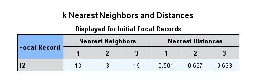
What is presented in this chart is the “ID” variable for the point that is currently selected. The three nearest neighbors, as measured through the utilization of the Euclidean distance formula. The Euclidean distances between the selected variable and the closest neighbor variables are presented in the rightmost portion of the chart.

Let’s now examine the data sheet output:

The rightmost column was added as a result of the option which we selected from the “Save” tab. What is being displayed in this new column, is the observational ID variable that is closest in proximity to the coinciding ID column when assessed through the utilization of the Euclidean distance formula.

Conclusion

What is the appropriate and applicable utilization of nearest neighbor? That question is mostly up to the end user. However, nearest neighbor analysis allows for the drawing of similarities between single observations of data. Suppose that we were trying to compare baseball players based on traditionally collected statistics, the above example would provide the perfect format for accomplishing such a task. In addition to being useful, the nearest neighbor function within SPSS provides beautiful output, which is impressive to any set of eyes.

That’s all for now, Data Heads! Stay subscribed for more interesting articles!