Keras differs from all of the other models in that it does not utilize the tree or forest methodologies as its primary mechanism of prediction. Instead, Keras employs something similar to a binary categorical method, in that, an observation is fed through the model, and at each subsequent layer prior to the output, Keras decides what the observation is, and what the observation is not. This may sound somewhat complicated, and in all manners, it truly is. However, what I am attempting to illustrate will become less opaque as you continue along with the exercise.
A final note prior to delving any further, Keras is a member of a machine learning family known as deep learning. Deep learning can essentially be defined as an algorithmic analysis of data which can evaluate non-linear relationships. This analysis also provides dynamic model re-calibration throughout the modeling process.
Keras Illustrated
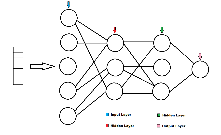
Below is a sample illustration of a Keras model which possesses a continuous dependent variable. The series of rows on the left represents the observational data which will be sent through the model so that it may “learn”. Each circle represents what is known as “neuron”, and each column of circles represents what is known as a “layer”. The sample illustration has 4 layers. The leftmost layer is known as the input layer, the middle two layers are known as the hidden layers, and the rightmost layer is referred to as the output layer.

How the Model Works
Without getting overly specific, (as many other resources exist which provide detailed explanations as it pertains the model’s inner-most mechanisms), the training of the model occurs throughout two steps. The first step being: “Forward Propagation”, and the second step being: “Backward Propagation”. Each node which exists beyond the input layers, sans the output layer, is measuring for a potential interaction amongst variables.
Each node is initially assigned a value. Those values shift as training data is processed through the model from the left to the right (forward propagation), and further, but more specifically modified, as the same data is then passed back through the model from the right to the left (back propagation). The entire training data set is not processed in its entirety in a simultaneous manner, instead, for the sake of allocating computing resources, the data is split into smaller sets known as batches. Batch size impacts learning significantly. With a smaller batch size, a model’s predictive capacity will be hindered. However, there are certain scenarios when lower batch size is advantageous, as the impact of noisy gradients will be reduced. The default size for a batch is 32 observations.
In many ways, the method in which the model functions is analogous to the way in which a clock operates. Each training observation shifts a certain aspect of a neuron’s value, with the neuron’s final value being representational of all of the prior shifts.
A few other terms which are also worth mentioning, as the selection of such is integral to model creation are:
Optimizer – This specifies the algorithm which will be utilized for correcting the model as errors occur.
Epoch – This indicates the number of times in which observational data will be passed through a model during the training process.
Loss Function – This indicates the algorithm which will be utilized to determine how errors are penalized within the model.
Metric - A metric is a function which is utilized to assess the performance of a model. However, unlike the Loss Function, it does not impact model training, and is only utilized to perform post-hoc analysis.
Model Application
As with any auxiliary python library, a library must first be downloaded and enabled prior to its utilization. To achieve this within the Jupyter Notebook platform, we will employ the following lines of code:
# Import ‘pip’ to import to install auxiliary packages #
import pip
# Install ‘TensorFlow’ to act as the underlying mechanism of the Keras UI #
pip.main(['install', 'TensorFlow'])
# Import pandas to enable data frame utilization #
import pandas
# Import numpy to enable numpy array utilization #
import numpy
# Import the general Keras library #
import keras
# Import tensorflow to act as the ‘backend’ #
import tensorflow
# Enable option for categorical analysis #
from keras.utils import to_categorical
from keras.models import Sequential
from keras.layers import Activation, Dense
# Import package to enable confusion matrix creation #
from sklearn.metrics import confusion_matrix
# Enable the ability to save and load models with the ‘load_model’ option #
from keras.models import load_model
# Enable the creation of confusion matrixes with the ‘sklearn.metrics’ library #
from sklearn.metrics import confusion_matrix
With all of the appropriate libraries downloaded and enabled, we can begin building our sample model.
Categorical Dependent Variable Model
For the following examples, we will be utilizing a familiar data set, the “iris” data set, which is available within the R platform.
# Import the data set (in .csv format), as a pandas data frame #
filepath = "C:\\Users\\Username\\Desktop\\iris.csv"
iris = pandas.read_csv(filepath)
First we will randomize the observations within the data set. Observational data should always be randomized prior to model creation.
# Shuffle the data frame #
iris = iris.sample(frac=1).reset_index(drop=True)
Next, we will remove the dependent variable entries from the data frame and modify the structure of the new data frame to consist only of independent variables.
predictors = iris.drop(['Species'], axis = 1).as_matrix()
Once this has been achieved, we must modify the variables contained within the original data set so that the categorical outcomes are designated by integer values.
This can be achieved through the utilization of the following code:
# Modify the dependent variable so that each entry is replaced with a corresponding integer #
from pandasql import *
pysqldf = lambda q: sqldf(q, globals())
q = """
SELECT *,
CASE
WHEN (Species = 'setosa') THEN '0'
WHEN (Species = 'versicolor') THEN '1'
WHEN (Species = 'virginica') THEN '2'
ELSE 'UNKNOWN' END AS SpeciesNum
from iris;
"""
df = pysqldf(q)
print(df)
iris0 = df
Next, we must make a few further modifications.
First, we must modify the dependent variable type to integer.
After such, we will identify this variable as being representative of a categorical outcome.
# Modify the dependent variable type from string to integer #
iris0['SpeciesNum'] = iris0['SpeciesNum'].astype('int')
# Modify the variable type to categorical #
target = to_categorical(iris0.SpeciesNum)
We are now ready to build our model!
# We must first specify the model type #
model = Sequential()
# Next, we will specify the output dimensions. This value will typically be [1] unless you are working with images. #
n_cols = predictors.shape[1]
# This next line specifies the traits of the input layer #
model.add(Dense(100, activation = 'relu', input_shape = (n_cols, )))
# This line specifies the traits of the hidden layer #
model.add(Dense(100, activation = 'relu'))
# This line specifies the traits of the output layer #
model.add(Dense(3, activation = 'softmax'))
# Compile the model by adding the optimizer, the loss function type, and the metric type #
# If the model’s dependent variable is binary, utilize the ‘binary_crossentropy' loss function #
model.compile(optimizer = 'adam', loss='categorical_crossentropy',
metrics = ['accuracy'])
With our model created, we can now go about training it with the necessary information.
As was the case with prior machine learning techniques, only a portion of the original data frame will be utilized to train the mode.
model.fit(predictors[1:100,], target[1:100,], shuffle=True, batch_size= 50, epochs=100)
With the model created, we can now test its effectiveness by applying it to the remaining data observations.
# Create a data frame to store the un-utilized observational data #
iristestdata = iris0[101:150]
# Create a data frame to store the model predictions for the un-utilized observational data #
predictions = model.predict_classes(predictors[101:150])
# Create a confusion matrix to assess the model’s predictive capacity #
cm = confusion_matrix(iristestdata['SpeciesNum'], predictions)
# Print the confusion matrix results to the console output window #
print(cm)
Console Output:
[[16 0 0]
[ 0 17 2]
[ 0 0 14]]
Continuous Dependent Variable Model
The utilization of differing model types is necessitated by the scenario that each situation dictates. As was the case with previous machine learning methodologies, the Keras package also contains functionality which allows for continuous dependent variables types.
The steps for applying this model methodology are as follows:
# Import the 'iris' data frame #
filepath = "C:\\Users\\Username\\Desktop\\iris.csv"
iris = pandas.read_csv(filepath)
# Shuffle the data frame #
iris = iris.sample(frac=1).reset_index(drop=True)
In the subsequent lines of code, we will first identify the model’s dependent variable ‘Sepal.Length’. This variable, and its corresponding observations will be held within the new variable ‘iris0’. Next, we will create the variable, ‘predictors’. This variable will be comprised of all of the variables contained within the ‘iris0’ data frame, with the exception of the ‘Sepal.Length’ variable. The new data frame will stored within a matrix format. Finally, we will again define the ‘n_cols’ variable.
target = iris['Sepal.Length']
# Drop Species Name #
iris0 = iris.drop(columns=['Species'])
# Drop Species Name #
predictors = iris0.drop(['Sepal.Length'], axis = 1).as_matrix()
n_cols = predictors.shape[1]
We are now ready to build our model!
# We must first specify the model type #
modela = Sequential()
# Next, we will specify the output dimensions. This value will typically be [1] unless you are working with images. #
n_cols = predictors.shape[1]
# This next line specifies the traits of the input layer #
modela.add(Dense(100, activation = 'relu', input_shape=(n_cols,)))
# This line specifies the traits of the hidden layer #
modela.add(Dense(100, activation = 'relu'))
# This line specifies the traits of the output layer #
modela.add(Dense(1))
# Compile the model by adding the optimizer and the loss function type #
modela.compile(optimizer = 'adam', loss='mean_squared_error')
With the model created, we must now train the model with the following code:
modela.fit(predictors[1:100,], target[1:100,], shuffle=True, epochs=100)
As was the case with the prior examples, we will only be utilizing a sample of the original data frame for the purposes of model training.
With the model created and trained, we can now test its effectiveness by applying it to the remaining data observations.
from sklearn.metrics import mean_squared_error
from math import sqrt
predictions = modela.predict(predictors)
rms = sqrt(mean_squared_error(target, predictions))
print(rms)
Model Functionality
In some ways, the Keras modeling methodology shares similarities with the hierarchal cluster model. The main differentiating factor being, in addition to the underlying mechanism, the dynamic aspects of the Keras model.
Each Keras neuron represents a relationship between independent data variables within the training set. These relationships exhibit macro phenomenon which may not be immediately observable within the context of the initial data. When finally providing an output, the model considers which macro phenomenon illustrated the strongest indication of identification. The Keras model still relies on generalities to make predictions, therefore, certain factors which are exhibited within the observational relationships are held in higher regard. This phenomenon is known as weighing, as each neuron is assigned a weight which is adjusted as the training process occurs.
The logistic regression methodology functions in a similar manner as it pertains to assessing variable significance. Again however, we must consider the many differentiating attributes of each model. In addition to weighing latent variable phenomenon, the Keras model is able to assess for non-linear relationships. Both attributes are absent within the aforementioned model, as logistic regression only assesses for linear relationships and can only provide values for variables explicitly found within the initial data set.
The sequential() model type, which was specified within the build process, is one of the many model options available within the Keras package. The sequential option differs from the other model types in that it creates a network in which each neuron within each layer, is connected to each neuron within each subsequent layer.

Other Characteristics of the Keras Model
Depending on the size of the data set which acted as the training data for the model, significant time may be required to re-generate a model after a session is terminated. To avoid this un-necessary re-generation process, functions exist which enable the saving and reloading of model information.
# Saving and Loading Model Data Requires #
from keras.models import load_model
# To save a model #
modelname.save("C:\\Users\\filename.h5")
# To load a model #
modelname = load_model("C:\\Users\\filename.h5")
It should be mentioned that as it pertains to Keras models, you do possess the ability to train existing models with additional data should the need the arise.
For instance, if we wished to train our categorical iris model (“model”) with additional iris data, we could utilize the following code:
model.fit(newpredictors[100:150,], newtargets[100:150,], shuffle=True, batch_size= 50, epochs=100)
There are errors which currently exist at the time of this article’s creation, which have yet to be resolved pertaining to learning rate fluctuation within re-loaded Keras models. Currently, a provisional fix has been suggested*, in which the "adam" optimizer is re-configured for re-loaded models. This re-configuring, while keeping all of the "adam" optimizer default configurations, significantly lowers the optimizer’s default learning rate. The purpose of this shift is to account for the differentiation in learning rates which occur in established models.
# Specifying Optimizer Traits Requires #
from keras import optimizers
# Re-configure Optimizer #
liladam = optimizers.adam(lr=0.00001, beta_1=0.9, beta_2=0.999, epsilon=None, decay=0.0, amsgrad=False)
# Utilize Custom Optimizer #
model.compile(optimizer = liladam, loss='categorical_crossentropy',
metrics = ['accuracy'])
*Source - https://github.com/keras-team/keras/issues/2378
Graphing Models
As we cannot easily determine the innermost workings of a Keras model, the best method of visualization can be achieved by graphing the learning output.
Prior to training the model, we will modify the typical fitting function to resemble something similar to the lines of code below:
history = model.fit(predictors[1:100,], target[1:100,], shuffle=True, epochs= 110, batch_size = 100, validation_data =(predictors[100:150,] , target[100:150,]))
What this code enables, is the creation of the data variable “history”, in which, data pertaining to the model training process will be stored. “validation_data” is instructing the python library to assess the specified data within the context of the model after each epoch. This does not impact the learning process. The way in which this assessment will be analyzed is determined by the selection of the “meteric” option specified within the model.fit() function.
If the above code is initiated, the model will be trained. To view the categories in which the model training history was organized upon being saved within the “history” variable, you may utilize the following lines of code.
history_dict = history.history
history_dict.keys()
This produces the console output:
dict_keys(['val_loss', 'val_acc', 'loss', 'acc'])
To set the appropriate axis lengths for our soon to be produced graph, we will initiate the following line:
epochs = range(1, len(history.history['acc']) + 1)
If we are utilizing Jupyter Notebook, we should also modify the graphic output size:
plt.rcParams["figure.figsize"] = [16,9]
We are now prepared to create our outputs. The first graphic can be prepared with the following code:
# Plot training & validation accuracy values #
# (This graphic cannot be utilized to track the validation process of continuous data models) #
plt.plot(epochs, history.history['acc'], 'b', label = 'Training acc')
plt.plot(epochs, history.history['val_acc'], 'bo', color = 'orange', label = 'Validation acc')
plt.title('Training and validation accuracy')
plt.ylabel('Loss')
plt.xlabel('Epoch')
plt.legend(loc='upper left')
plt.show()
This produces the output:

What this graphic is illustrating, is the level of accuracy in which the model predicts results. The solid blue line represents the data which was utilized to train the model, and the orange dotted line represents the data which is being utilized to test the model’s predictability. It should be evident that throughout the training process, the predictive capacity of the model improves as it pertains to both training and validation data. If a large gap emerged, similar to the gap which is observed from epoch # 20 to epoch # 40, we would assume that this divergence of data is indicative of “overfitting”. This term is utilized to describe a model which can predict training results accurately, but struggles to predict outcomes when applied to new data.
The second graphic can be prepared with the following code:
# Plot training & validation loss values
plt.plot(epochs, history.history['loss'], 'b', label = 'Training loss')
plt.plot(epochs, history.history['val_loss'], 'bo', label = 'Validation loss', color = 'orange')
plt.title('Training and validation loss')
plt.ylabel('Loss')
plt.xlabel('Epoch')
plt.legend(loc='upper left')
plt.show()

This graphic is illustrates the improvement of the model over time. The solid blue line represents the data which was utilized to train the model, and the orange dotted line represents the data which is being utilized to test the model’s predictability. If a gap does not emerge between the lines throughout the training process, it is advisable to set the number of epochs to a figure which, after subsequent graphing occurs, demonstrates a flat plateauing of both lines.
Reproducing Model Training Results
If Keras is being utilized, and TensorFlow is the methodology selected to act as a “backend”, then the following lines of code must be utilized to guarantee reproductivity of results.
# Any number could be utilized within each function #
# Initiate the RNG of the general python library #
import random
# Initiate the RNG of the numpy package #
import numpy.random
# Set a random seed as it pertains to the general python library #
random.seed(777)
# Set a random seed as it pertains to the numpy library #
numpy.random.seed(777)
# Initiate the RNG of the tensorflow package #
from tensorflow import set_random_seed
# Set a random seed as it pertains to the tensorflow library #
set_random_seed(777)
Missing Values in Keras
Much like the previous models discussed, Keras has difficulties as it relates to variables which contain missing observational values. If a Keras model is trained on data which contains missing variable values, the training process will occur without interruption, however, the missing values will be analyzed under the assumption that they are representative of a measurement. Meaning, that the library will NOT automatically assume that the value is a missing value, and from such, estimate a place holder value based on other variable observations within the set.
To make assumptions for the missing values based on the process described above, we must utilize the imputer() function from the python library: “sklearn”. Sample code which can be utilized for this purpose can be found below:
from sklearn.preprocessing import Imputer
imputer = Imputer()
transformed_values = imputer.fit_transform(predictors)
Additional details pertaining to this function, its utilization, and its underlying methodology, can be found within the previous article: “(R) Machine Learning - The Random Forest Model – Pt. III”.
Having tested this method of variable generation on sets which I purposely modified, I can attest that its capability for achieving such is excellent. After generating fictitious placeholder values and then subsequently utilizing the Keras package to create a model, comparatively speaking, I saw no differentiation between the predicted results related to each individual set.
Early Stopping
There may be instances which necessitate the creation of a model that will be applicable to a very large data set. This essentially, in most cases, guarantees a very long training time. To help assist in shortening this process, we can utilize an “early stopping monitor”.
First, we must import the package related to this feature:
from keras import losses
Next we will create and define the parameters pertaining to the feature:
# If model improvement stagnates after 2 epochs, the fitting process will cease #
early_stopping_monitor = keras.callbacks.EarlyStopping(monitor='loss', patience = 2, min_delta=0, verbose=0, mode='auto', baseline=None, restore_best_weights=True)
Many of the options present within the code above are defaults. However, there are few worth mentioning.
monitor = ‘loss’ - This option is specifically instructing the function to monitor the loss value during each training epoch.
patience = 2 – This option is instructing the function to cease training if the loss value ceases to decline after 2 epochs.
restore_best_weights=True – This option is indicating to the function that the values which occurred prior to lack of loss within the training process, should be the last values applied as it pertains to model training. The subsequent training values will be discarded.
With the early stopping feature defined, we can add it to the training function below:
history = model.fit(predictors[101:150,], target[101:150,], shuffle=True, epochs=100, callbacks =[early_stopping_monitor], validation_data =(predictors[100:150,] , target[100:150,]))
Final Thoughts on Keras
In my final thoughts pertaining to the Keras model, I would like to discuss the pros and cons of the methodology. Keras is, without doubt, the machine learning model type which possesses the greatest predictive capacity. Keras can also be utilized to identify images, which is a feature that is lacking within most other predive models. However, despite these accolades, Keras does fall short in a few categories.
For one, the mathematics which act a mechanism for the model’s predicative capacity are incredibly complex. As a result of such, model creation can only occur within a digital medium. With this complexity comes an inability to easily verify or reproduce results. Additionally, creating the optimal model configuration as it pertains to the number of neurons, layers, epochs, etc., becomes almost a matter of personal taste. This sort of heuristic approach is negative for the field of machine learning, statistics, and science in general.
Another potential flaw relates to the package documentation. The website for the package is poorly organized. The videos created by researchers who attempt to provide instruction are also poorly organized, riddled with heuristic approach, and scuttled by a severe lack of awareness. It would seem that no single individual truly understands how to appropriately utilize all of the features of the Keras package. In my attempts to properly understand and learn the Keras package, I purchased the book, DEEP LEARNING with Python, written by the package’s creator, Francois Chollet. This book was also poorly organized, and suffered from the assumption that the reader could inherently understand the writer’s thoughts.
This being said, I do believe that the future of statistics and predictive analytics lies parallel with the innovations demonstrated within the Keras package. However, the package is so relatively new, that not a single individual, including the creator, has had the opportunity to utilize and document its potential. In this lies latent opportunity for the patient individual to prosper by pioneering the sparse landscape.
It is my opinion that at this current time, the application of the Keras model should be paired with other traditional statistical and machine learning methodologies. This pairing of multiple models will enable the user and potential outside researchers to gain a greater understanding as to what may be motivating the Keras model’s predictive outputs.
No comments:
Post a Comment
Note: Only a member of this blog may post a comment.