Monday, October 16, 2023

The Friendship Paradox

Like many of the critical attributes of life, that which is most evident, lies obscured by monotony. This is especially true as it pertains to mathematical paradoxes, as the most enlightening insights within the field, have the habit of appearing both obvious and universally evident after discovery. Like many mystical traditions, these insights are best discovered through contradiction and reduction.

The Paradox

The Friendship Paradox, in simpler terms, identifies the common phenomenon in which an individual, typically possesses less friends than his friends. Additionally, the sum of friends which his friends possess, will be greater than the sum of his total number of friends.

This paradox possesses wide reaching implications, as it describes events which are self-arising and irrefutable. However, before we can detail applicability, we must demonstrate the paradox as it was initially discerned.

First, let’s get some terminology down.

In graph theory, circular graphics are known as nodes, or vertexes. The lines which illustrate relationships between the nodes are known as edges.


Now, let’s utilize this style of graphical representation to demonstrate the relationships between 5 individuals.


The chart below represents the above relationships, but in a different format.


As each relationship is symmetric, if one friend considers himself to be a friend of another individual, that individual also considers the initial individual to be his friend as well. As shown above, A is friends with B and E. B is friends with both A and E, and also friends with C.

If we derive the mean as it relates to the average number of friends that an individual possesses within our experiment, we come to the value of 2.8.


In this instance, E possesses the most friends, and every individual who is friends with E, possesses less. Therefore, the average number of friends that an individual within a group possesses (2.8), will likely be greater than the actual number of friends that a singular individual possesses. 

The Philosophical Implications   

If a single individual begins to quantify a particular phenomenon as it relates to their person on an individualized basis, or even as it relates to a novel phenomenon, then the natural consequence of this endeavor is that this individual from the onset will find himself at a disadvantage.

For example, a new creation upon its genesis, possessing autonomy, will immediately be concerned with attaining sustenance. This was not a concern which was possessed within the prior state of non-being. In contemplating one’s beauty, a young woman immediately begins to compare herself to those whom she perceives as being more beautiful. We would never anticipate the inverse to occur.

This is the paradox of living, striving to possess more while the value of that which we possess becomes diminished. This is due to the passage of time, but also due to singular possession of a resource also diminishing in value. Something within our possession loses value from the moment of possession, as both the individual and the possession are diminished by the natural passage of time.

Example (2):

Here is another example, if an individual walks into a crowded elevator filled with random strangers, then there is a greater probability that this individual will have the same number, or a greater number of friends, than each stranger within the elevator. However, if the same individual were invited to a party hosted by a friend, then there is a lesser probability of this individual possessing more friends, or a similar number of friends, as compared to each other party attendees. In the elevator scenario, there is no guarantee that any individual within the elevator possesses a single friend. This also includes the individual entering the already crowded elevator. However, in the party scenario, each party goer has at least one friend, that being - the party’s host. In this case, the count begins at the neutral value of 1, except for the case of the party’s host, who is friends with every individual in attendance.

As described above, the friendship paradox also seeks to demonstrate, “the sum of friends which his friends possess, will be greater than the sum of his total number of friends.”

In the case of our first example, this value would be calculated as follows:


To better illustrate this phenomenon, I’ve constructed a new example relationship diagram below:


In this instance, E has more friends than A, B, C, D.

E has 4 friends. While A, B, C, D each have 1 friend (E).

In total: A, B, C, D possess the same number of friends in sum (1+1+1+1).

If A, B, C, or D possessed one additional friend – F, then in total, they would together possess more friends in sum than E (1 + 1 + 1 + 2).

If this were the case, the paradox would hold, as E would have a total of 4 friends, but the total number of his friends of friends would be greater (5).

Conclusion

That's all for today.

I hope that you enjoyed this entry and will visit again soon.

-RD

(R) Utilizing Crowd Prediction Methodologies to Draft the Optimal Fantasy Football Team (II)

What would an application be without proof? A notion?

To prove that the ADP drafting strategy is superior to other ranking methodologies, I performed the following analysis.

#############################################################################

Data Source(s):

#############################################################################


ADP

https://fantasydata.com/nfl/fantasy-football-leaders?position=1&season=2022&seasontype=1&scope=1&subscope=1&scoringsystem=2&startweek=1&endweek=1&aggregatescope=1&range=1

Offense

https://fantasydata.com/nfl/ppr-adp?season=2022&leaguetype=2&type=ppr

Kickers

https://fantasydata.com/nfl/fantasy-football-leaders?position=6&season=2022&seasontype=1&scope=1&subscope=1&scoringsystem=2&startweek=1&endweek=1&aggregatescope=1&range=1

DST

https://fantasydata.com/nfl/fantasy-football-leaders?position=7&season=2022&seasontype=1&scope=1&subscope=1&scoringsystem=2&startweek=1&endweek=1&aggregatescope=1&range=1

#############################################################################

The Analysis (n = 300)

#############################################################################


ADP <- c(1.4, 2.4, 2.7, 4.2, 4.9, 5.8, 7, 7.2, 8.8, 10, 10.6, 12.4, 13.1, 14, 15.3, 16, 16.6, 17.9, 18.5, 19.1, 19.6, 19.8, 21.8, 22.7, 24.7, 25.9, 26.1, 27.3, 27.9, 29.3, 30.5, 31.6, 32.4, 33.2, 33.2, 34.1, 36.1, 38, 39.1, 39.3, 39.4, 39.7, 42.3, 43.2, 43.5, 44.2, 45.1, 46.5, 46.8, 47.3, 48.4, 50.2, 50.9, 51.5, 52.2, 53.9, 54.1, 56, 56.7, 57.9, 59.4, 61.2, 61.5, 62.1, 62.9, 63, 63.8, 63.9, 68, 68.1, 69.2, 69.9, 70.1, 71, 71.4, 71.7, 72, 72.9, 75.3, 75.4, 77.1, 77.9, 82.3, 83.8, 84.4, 84.8, 85, 86.7, 87.9, 89.5, 90.2, 90.2, 90.7, 91.3, 91.7, 91.8, 94.4, 95.9, 96.2, 98.5, 98.7, 99.1, 101.9, 102.6, 102.7, 103.6, 103.7, 105.4, 106.5, 106.7, 107.8, 108.6, 109.7, 109.9, 110.6, 111.6, 113.1, 113.6, 113.9, 114.9, 117.3, 117.7, 118.5, 119, 119.6, 120.5, 121, 121.2, 121.3, 122.7, 124.2, 125, 128.9, 129.8, 130.2, 130.2, 130.3, 130.8, 131.2, 132, 135.1, 135.9, 136.1, 136.3, 137.9, 138.9, 140.1, 140.9, 141.8, 142.7, 143.8, 144.8, 145.3, 145.4, 145.7, 147, 147, 148.1, 148.4, 148.9, 149, 149.4, 151.3, 151.4, 152.1, 152.5, 152.6, 153.8, 154.9, 155.6, 155.7, 156.7, 156.8, 156.8, 158, 158.5, 158.8, 158.9, 159.4, 160.1, 160.5, 160.7, 161, 161.5, 162, 163, 163.5, 164, 164.6, 164.6, 165, 165.2, 165.6, 166, 167, 168, 169, 169.5, 170, 171, 172, 173, 174, 175, 176, 177, 178, 178, 179, 180, 180, 181, 182, 183, 184, 185, 186, 187, 187, 188, 189, 190, 190, 191, 192, 192, 193, 193, 194, 195, 196, 197, 198, 199, 200, 201, 202, 203, 204, 205, 206, 207, 208, 209, 210, 211, 212, 213, 214, 215, 216, 217, 218, 219, 220, 221, 222, 223, 224, 225, 226, 227, 228, 229, 230, 231, 232, 233, 234, 235, 236, 237, 238, 239, 240, 241, 242, 243, 244, 245, 246, 247, 248, 249, 250, 251, 252, 253, 254, 255, 256, 257, 258, 259, 260, 261, 262, 263, 264, 265)


PPR <- c(146.4, 356.36, 372.7, 302.76, 368.66, 201.4, 223.46, 237.8, 242.4, 239.5, 211.7, 335.5, 191.1, 316.6, 248.6, 284, 316.3, 301.6, 281.4, 395.52, 168.4, 42, 226.1, 347.2, 216.5, 190.5, 225.4, 185.8, 200.2, 164, 299.6, 75.6, 220.9, 281.26, 141.3, 205.1, 199.1, 229, 417.4, 177.7, 81.2, 176.5, 43.6, 200.5, 180.7, 115.1, 159.4, 259.2, 350.7, 328.3, 167.6, 84.8, 226.8, 236.08, 51.1, 84.9, 98.3, 378.04, 222.8, 145.6, 90.9, 204.2, 216.7, 200.52, 142.7, 52.2, 171.6, 180, 156, 101.5, 126.8, 248.8, 74.2, 166.4, 79, 177.9, 225.76, 267.6, 141.2, 185.3, 249.1, 239.2, 53.5, 246, 87.1, 198.6, 254.6, 271.66, 88.1, 115.6, 227.8, 151.7, 174.8, 105.7, 108.38, 148.7, 69.4, 202.5, 241.9, 88.6, 148.2, 12.46, 168.3, 219.08, 115.7, 178.6, 147.3, 57.3, 87.9, 159.4, 291.58, 55.8, 198.2, 112.7, 237.3, 126, 98.2, 73.5, 135.7, 165.9, 150, 43.4, 135, 105.4, 215.4, 225.9, 70.4, 230.92, 167.12, 139.1, 166.5, 87.7, 88.4, 102, 122.4, 7, 94.1, 114, 105.04, 155.28, 102.9, 160, 103.9, 101.6, 159, 102, 98, 161, 295.98, 295.62, 115, 87.9, 112, 133, 101, 103, 55.2, 43.92, 116, 97, 131, 180.3, 121, 130.6, 143, 142, 119.8, 215.7, 25.5, 125, 123.6, 99, 39, 110, 97.1, 130, 129, 97, 57, 18, 118, 154, 168, 100, 116.9, 20.1, 104, 98.2, 186, 97, 60.2, 110, 101, 52.2, 155.6, 93.8, 3.2, 110, 169.3, 97.6, 34.4, 161.1, 78.9, 25.8, 51.6, 112.3, 115, 176.3, 198.1, 106, 26.4, 82.7, 149.1, 117.8, 88.3, 81.7, 110.1, 83, 4.5, 50.1, 164.1, 73, 12, 57.68, 139, 61.6, 112, 77.4, 45.4, 46.5, 15.1, 35.5, 72.7, 75.2, 84.5, 110, 0.2, 142.1, 34, 12.2, 83, 82.6, 21.1, 77.2, 196.3, 11.4, 51.7, 8.4, 54.1, 161.24, 46.2, 8.6, 8.4, 13.8, 289, 37.8, 170.08, 128.4, 89.6, 112.8, 104.1, 284.32, 154.16, 59.3, 24.9, 114.5, 121.42, 158.5, 59.8, 98.92, 0, 115.1, 10.2, 181.52, 14.8, 4.2, 12.8, 18.8, 103.9, 196.56, 1.3, 11.8, 16.2, 26, 39.1, 43.1, 53.6, 103.8, 27.3, 303.88, 30.8, 64.5, 3.5, 73.88, 110.2, 64.7, 84.3, 30.5, 10.2, 70.3)

cor.test(ADP, PPR)

Which produces the output:

Pearson's product-moment correlation

data: ADP and PPR

t = -13.394, df = 298, p-value < 2.2e-16

alternative hypothesis: true correlation is not equal to 0

95 percent confidence interval:

-0.6791003 -0.5370390

sample estimates:

cor

-0.6130004


#############################################################################

Creating the Visual Output

#############################################################################


my_data <- data.frame(ADP, PPR)

library("ggpubr")

ggscatter(my_data, x = "ADP", y = "PPR",

add = "reg.line", conf.int = TRUE,

cor.coef = TRUE, cor.method = "pearson",

xlab = "ADP (2022)", ylab = "Player Score (PPR)")

#############################################################################

Conclusion

#############################################################################


There was a negative correlation between the two variables: ADP (n = 300), and Player Score (PPR). ADP (M = 134.81, SD = 73.31), Player Score (PPR) (M = 133.33, SD = 86.66), Conditions; t(298) = -13.394 , p < .01. Pearson Product-Moment Correlation Coefficient: r = -0.61.

#############################################################################

As the findings indicate, there is a significant negative correlation as it pertains to ADP and player performance (PPR - 2022 Season). In plain terms, this means that we should typically expect to see better fantasy performance from players with lower ADP rankings. I hope that everyone enjoyed this article and my adherence to APA reporting standards. <3

Until next time. 

Stay cool, Data Heads.

-RD

Monday, October 9, 2023

Utilizing Crowd Prediction Methodologies to Draft the Optimal Fantasy Football Team

To win your league in Fantasy Football, or at least qualify for the playoffs, you don’t need to buy magazines, study tape, or watch ESPN. All that is required, is a general understanding of crowd psychology.

What is ADP?

ADP represents the average draft position for players in fantasy drafts. Each league, for each fantasy sport, typically displays this player value during the drafting process. This value, as the name suggests, is derived from where a particular player was selected by other “fantasy team owners”, during prior drafts.

As was discussed within a previous article demonstrating draft order and its impact on a fantasy team’s final placement, if each fantasy team owner drafted optimally within their respective position, we would expect the final standings to directly reflect the initial draft order.

However, how can an individual be sure that he is drafting optimally? The answer is simpler than one might assume. To achieve optimal drafting potential, one must adhere to drafting players with the best available ADP value throughout the drafting process.

Why does it Work?

Following the crowd consensus, should provide a fantasy participant with their best opportunity for victory. The strictest adherent to this methodology, will benefit most from the number non-adherents within their league. Let’s consider why this is the case.

While pundit, or site rankings of players are often determined by a single individual, or a group of informed individuals, ADP rankings are determined by draft consensus. Meaning, that there are more minds at work as it pertains to determining a player’s draft value. These ranks are also assigned through the drafting process. This differs from other ranking processes, in that, the act of drafting establishes the value. This is similar as to how market participants set prices through buying and selling assets. Whereas, the ranking process is more akin to the way in which planned economies function.   

We’ll assume that ADP perfectly correlates with the eventual points scored by each player within the league. Therefore, with this assumption in place, and also assuming that each league participant drafts optimally, we should expect to see point distributions resemble something like the graphic below. 


(In our example scenario, each subsequent player is valued at one point less than the previous player.)

Therefore, all things being equal, we would expect the final point totals for each league participant to be:


Gaining the Edge

In every instance, the largest advantage belongs to the team which drafts first, with diminishing advantage being assessed sequentially throughout the remaining draft order. To attempt to compensate for this diminishment, or to expand one’s edge regardless of draft position, a league participant should strongly adhere to the ADP value ranking system while drafting. By not attempting to gain an edge through self perceived insight, opportunities will arise as a result of opponents who attempt otherwise.

Every draft misstep is the micro-process of reallocating points from your team to another team within your league. In the example below, the teams highlighted in green are adhering to a strict ADP drafting strategy. The teams highlighted in red, instead are going for a less strict approach.


As is shown in the graphic, the ADP adhering teams were able to benefit from the mistakes made by their opponents. In each instance, the green teams were able to draft the players which were passed upon by their red counterparts. Thus, the ADP adhering teams increased their edge at the expense of the non-adhering teams.


I Know that I Know Nothing


The above strategy, functions on the foundation of two re-enforcing cognitive biases. One being the overestimation of one’s own abilities and talents, and the other being the discounting of the abilities and talents of others.

As far as football is concerned, I have personally witnessed friends who watch far more football than I do, who know far more about the players than I do, blow out their drafts, and fail to make their league’s playoffs in complex and interesting ways. In almost every case, the culprit tends to be impatience and exotic maneuvering. What’s also strange about this cohort of individuals, is that they tend to quickly abandon the strange individualized strategies which initially required a high level of conviction to attempt. This phenomenon itself might warrant an article in the future. 

Be sure to watch the waiver wire, as further edge can be gained from managers who prematurely release underperforming players. Also, it should be noted, that ADP rankings as a drafting criteria, are only applicable in leagues which do not utilize custom rule sets.

Sunday, July 23, 2023

Odd Man Out: The Problem with Serpentine Drafts

In this article, we’re going to continue the trend of discussing topics related to Fantasy Sports. Specifically, the innate problem which I see within the serpentine draft format. I feel that this topic is particularly appropriate for this time of year, as football fans are gearing up for their own fantasy league drafts.

If you’re unfamiliar with the serpentine draft format, it is best described as:

A serpentine draft, or sometimes referred to as a a "Snake" draft, is a type in which the draft order is reversed every round (eg 1..12, 12..1, 1..12, 12..1, etc.). For example, if you have the first pick in the draft, you will pick first in round one, and then last in round two.

Source: https://help.fandraft.com/support/solutions/articles/61000278703-draft-types-and-formats

I’ve created a few examples of this draft type below. The innate issue which I see within this draft format, pertains to the differentiation between the projected point value of each draft selection, as determined by a team’s draft position. The more teams present within a league, the greater the point disparity between teams.

Assuming that each team executed an optimized drafting strategy, we would expect the outcome to resemble something like the illustration below.

Each number within a cell represents the best player value available to each team, each round. The green cells contain starting player values, and the grey cells contain back-up player values.


As you can observe from the summed values below each outcome column, each team possess a one point advantage against the team which selected subsequently, and a one point disadvantage against the team which selected previously. The greatest differentiation occurring between the team which made the first selection within the draft order, as measured against the team which made the last selection within the draft order: 11 (1026 – 1015).

As previously mentioned, the less teams within a league, the less the number of selection rounds. As a result of such, there is less of a disparity between the teams which pick earlier within the order, as compared to teams which pick later within the order.

Below is the optimal outcome of a league comprised of ten teams.


While the single point differentiation persists between consecutive teams within the draft order, the differentiation between the first selector, and the last selector, has been reduced to: 9 (856 – 847).

This trend continues across ever smaller league sizes: 7 (1024 – 1017).


In each instance, we should expect the total differentiation of points between the first draft participant, and last draft participant, (if optimal drafting occurred), to be equal to: N – 1. Where N = the number of total draft participants within the league.

All things being equal, if each team is managed optimally, we should expect the first team within each draft to finish first within each league. Second place would belong to the team which drafted second. Third place belonging to the team which drafted third, and so on, etc.

If all players are equally at risk of being injured on each fantasy team, then this occurrence does little to upset the overall ranking of teams by draft order. It must be remembered that teams which drafted earlier within the order, will also possess better replacement players as compared to their competitors. Therefore, when injuries do occur, later drafting teams will be disproportionately impacted.

I would imagine that as AI integration begins to seep into all aspects of existence, that the opportunity for each team owner to draft with consistent optimization, will further stratify the inherent edge attributed to serpentine draft position. As it stands currently, there is still an opportunity for lower draft order teams to compete if one or more of their higher order competitors blunder a selection. 

In any case, I hope that what I have written in this article helped to describe what I like to refer to as the, “Odd Man Out” phenomenon. I hope to see you again soon, with more of the statistical content which you crave.

-RD

Monday, July 17, 2023

(R) Daily Fantasy Sports Line-up Optimizer (Basketball)

I’ve been mulling over whether or not I should give away this secret sauce on my site, and I’ve come to the conclusion that anyone who seriously contends within the Daily Fantasy medium, probably is already aware of this strategy. 

Today, through the magic of R software, I will demonstrate how to utilize code to optimize your daily fantasy sports line-up. This particular example will be specific to the Yahoo daily fantasy sports platform, and to the sport of basketball.

I also want to give credit, where credit is due.

The code presented below is a heavily modified variation of code initially created by: Patrick Clark.

The original code source case be found here: http://patrickclark.info/Lineup_Optimizer.html

Example:

First, you’ll need to access Yahoo’s Daily Fantasy page. I’ve created an NBA Free QuickMatch, which is a 1 vs. 1 contest against an opponent where no money changes hands.


This page will look a bit different during the regular season, as the NBA playoffs are currently underway. That aside, our next step is to download all of the current player data. This can be achieved by clicking on the “i” bubble icon.


Next, click on the “Export players list” link. This will download the previously mentioned player data.

The player data should resemble the (.csv) image below:


Prior to proceeding to the subsequent step, we need to do a bit of manual data clean up.

Any player who is injured or not starting, I removed from the data set. I also concatenated the First Name and Last Name fields, and placed that concatenation within the ID variable. Next, I removed all variables except for the following: ID (newly modified), Position, Salary, and FPPG (Fantasy Points Per Game).

The results should resemble the following image:


(Specific player data and all associated variables will differ depending on the date of download)

Now that the data has been formatted, we’re ready to code!

###################################################################

library(lpSolveAPI)

library(tidyverse)

# It is easier to input the data as an Excel file if possible #

# Player names (ID) have the potential to upset the .CSV format #

library(readxl)

# Be sure to set the played data file path to match your directory / file name #

PlayerPool <- read_excel("C:/Users/Your_Modified_Players_List.xlsx")

# Create some positional identifiers in the pool of players to simplify linear constraints #

# This code creates new position column variables, and places a 1 if a player qualifies for a position #

PlayerPool$PG_Check <- ifelse(PlayerPool$Position == "PG",1,0)

PlayerPool$SG_Check <- ifelse(PlayerPool$Position == "SG",1,0)

PlayerPool$SF_Check <- ifelse(PlayerPool$Position == "SF",1,0)

PlayerPool$PF_Check <- ifelse(PlayerPool$Position == "PF",1,0)

PlayerPool$C_Check <- ifelse(PlayerPool$Position == "C",1,0)

PlayerPool$One <- 1

# This code modifies the position columns so that each variable is a vector type #

PlayerPool$PG_Check <- as.vector(PlayerPool$PG_Check)

PlayerPool$SG_Check <- as.vector(PlayerPool$SG_Check)

PlayerPool$SF_Check <- as.vector(PlayerPool$SF_Check)

PlayerPool$PF_Check <- as.vector(PlayerPool$PF_Check)

PlayerPool$C_Check <- as.vector(PlayerPool$C_Check)

# This code orders each player ID by position #

PlayerPool <- PlayerPool[order(PlayerPool$PG_Check),]

PlayerPool <- PlayerPool[order(PlayerPool$SG_Check),]

PlayerPool <- PlayerPool[order(PlayerPool$SF_Check),]

PlayerPool <- PlayerPool[order(PlayerPool$PF_Check),]

PlayerPool <- PlayerPool[order(PlayerPool$C_Check),]

# Appropriately establish variables in order to perform the "solver" function #

Num_Players <- length(PlayerPool$One)

lp_model = make.lp(0, Num_Players)

set.objfn(lp_model, PlayerPool$FPPG)

lp.control(lp_model, sense= "max")

set.type(lp_model, 1:Num_Players, "binary")

# Total salary points avalible to the player #

# In the case of Yahoo, the salary points are set to ($)200 #

add.constraint(lp_model, PlayerPool$Salary, "<=",200)

# Maximum / Minimum Number of Players necessary for each position type #

add.constraint(lp_model, PlayerPool$PG_Check, "<=",3)

add.constraint(lp_model, PlayerPool$PG_Check, ">=",1)

# Maximum / Minimum Number of Players necessary for each position type #

add.constraint(lp_model, PlayerPool$SG_Check, "<=",3)

add.constraint(lp_model, PlayerPool$SG_Check, ">=",1)

# Maximum / Minimum Number of Players necessary for each position type #

add.constraint(lp_model, PlayerPool$SF_Check, "<=",3)

add.constraint(lp_model, PlayerPool$SF_Check, ">=",1)

# Maximum / Minimum Number of Players necessary for each position type #

add.constraint(lp_model, PlayerPool$PF_Check, "<=",3)

add.constraint(lp_model, PlayerPool$PF_Check, ">=",1)

# Maximum / Minimum Number of Players necessary for each position type (only require one (C)enter) #

add.constraint(lp_model, PlayerPool$C_Check, "=",1)

# Total Numner of Players Needed for the entire Fantasy Line-up #

add.constraint(lp_model, PlayerPool$One, "=",8)

# Perform the Solver function #

solve(lp_model)

# Projected_Score provides the projected score summed from the optimized projected line-up (FPPG) #

Projected_Score <- crossprod(PlayerPool$FPPG,get.variables(lp_model))

get.variables(lp_model)

# The optimal_lineup data frame provides the optimized line-up selection #

optimal_lineup <- subset(data.frame(PlayerPool$ID, PlayerPool$Position, PlayerPool$Salary), get.variables(lp_model) == 1)


If we take a look at our:

Projected_Score

We should receive an output which resembles the following:

> Projected_Score
    [,1]
[1,] 279.5

Now, let’s take a look at our:

optimal_lineup

Our output should resemble something like:

PlayerPool.ID PlayerPool.Position PlayerPool.Salary
3 Marcus Smart PG 20
51 Bradley Beal SG 43
108 Tyrese Haliburton SG 16
120 Jerami Grant SF 27
130 Eric Gordon SF 19
148 Brandon Ingram SF 36
200 Darius Bazley PF 19
248 Steven Adams C 20

With the above information, we are prepared to set our line up.

You could also run this line of code:

optimal_lineup <- subset(data.frame(PlayerPool$ID, PlayerPool$Position, PlayerPool$Salary, PlayerPool$FPPG), get.variables(lp_model) == 1)

optimal_lineup


Which provides a similar output that also includes point projections:

PlayerPool.ID PlayerPool.Position PlayerPool.Salary PlayerPool.FPPG
3 Marcus Smart PG 20 29.8
51 Bradley Beal SG 43 50.7
108 Tyrese Haliburton SG 16 26.9
120 Jerami Grant SF 27 38.4
130 Eric Gordon SF 19 30.7
148 Brandon Ingram SF 36 43.2
200 Darius Bazley PF 19 29.7
248 Steven Adams C 20 30.1

Summing up PlayerPool.FPPG, we reach the value: 279.5. This was the same value which we observed within the Projected_Score matrix.

Conclusion:

While this article demonstrates a very interesting concept, I would be remiss if I did not advise you to NOT gamble on daily fantasy. This post was all in good fun, and for educational purposes only. By all means, defeat your friends and colleagues in free leagues, but do not turn your hard-earned money over to gambling websites.

The code presented within this entry may provide you with a minimal edge, but shark players are able to make projections based on far more robust data sets as compared to league FPPG. 

In any case, the code above can be repurposed for any other daily fantasy sport (football, soccer, hockey, etc.). Remember, only to play for fun and for free. 

-RD 

Sunday, July 9, 2023

(R) Bedford's Law

In today’s article, we will be discussing Benford’s Law, specifically as it is utilized as an applied methodology to assess financial documents for potential fraud:

First, a bit about the phenomenon which Benford sought to describe:

The discovery of Benford's law goes back to 1881, when the Canadian-American astronomer Simon Newcomb noticed that in logarithm tables the earlier pages (that started with 1) were much more worn than the other pages. Newcomb's published result is the first known instance of this observation and includes a distribution on the second digit, as well. Newcomb proposed a law that the probability of a single number N being the first digit of a number was equal to log(N + 1) − log(N).

The phenomenon was again noted in 1938 by the physicist Frank Benford, who tested it on data from 20 different domains and was credited for it. His data set included the surface areas of 335 rivers, the sizes of 3259 US populations, 104 physical constants, 1800 molecular weights, 5000 entries from a mathematical handbook, 308 numbers contained in an issue of Reader's Digest, the street addresses of the first 342 persons listed in American Men of Science and 418 death rates. The total number of observations used in the paper was 20,229. This discovery was later named after Benford (making it an example of Stigler's law).


Source: https://en.wikipedia.org/wiki/Benford%27s_law

So what does this actually mean in laymen’s terms?

Essentially, given a series of numerical elements from a similar source, we should expect certain leading digits to occur, and correspond to, a particular distribution patter. 


If a series of elements perfectly corresponds with Benford’s Law, then the elements within the series should follow the above pattern as it pertains to leading digit frequency. Ex. Numbers which begin the number “1”, should occur 30.1% of the time. Numbers which begin with the number “2”, should occur 17.6% of the time. Numbers which begin with the number “3”, should occur 12.5% of the time.

The distribution is derived as follows:


The utilization of Benford’s Law is applicable to numerous scenarios:

1. Accounting fraud detection

2. Use in criminal trials

3. Election data 

4. Macroeconomic data

5. Election data 

6. Price digit analysis 

7. Genome data 

8. Scientific fraud detection 

As it relates to screening for financial fraud, if the application of methodology related to the Benford’s Law Distribution returns a result in which the sample elements do not correspond with the distribution, then fraud is not necessarily the conclusion which we would immediately assume. However, the findings may indicate that additional data scrutinization is necessary. 

Example:

Let’s utilize Benford’s Law to analyze Cloudflare’s (NET) Balance Sheet (12/31/2021).


Even though it’s an un-necessary step as it relates to our analysis, let’s first discern the frequency of each leading digit. These digits are underlined in red within the graphic above.


What Benford’s Law will seeks to assess, is the comparison of leading digits as they occurred within our experiment, to our expectations as they exist within the Benford’s Law Distribution.


The above table illustrates the frequency of occurrence of each leading digit within our analysis, versus the expected percentage frequency as stated by Benford’s Law.

Now let’s perform the analysis:

# H0: The first digits within the population counts follow Benford's law #

# H1: The first digits within the population counts do not follow Benford's law #

# requires benford.analysis #

library(benford.analysis)

# Element entries were gathered from Cloudflare’s (NET) Balance Sheet (12/31/2021) #

NET <- c(2372071.00, 1556273.00, 815798.00, 1962675.00, 815798.00, 134212.00, 791014.00, 1667291.00, 1974792.00, 791014.00, 1293206.00, 845217.00, 323612.00, 323612.00)

# Perform Analysis #

trends <- benford(NET, number.of.digits = 1, sign = "positive", discrete=TRUE, round=1)

# Display Analytical Output #

trends

# Plot Analytical Findings #

plot(trends)


Which provides the output:

Benford object:

Data: NET
Number of observations used = 14
Number of obs. for second order = 10
First digits analysed = 1

Mantissa:

Statistic Value
    Mean 0.51
    Var 0.11
Ex.Kurtosis -1.61
    Skewness 0.25

The 5 largest deviations:

digits absolute.diff
1 8 2.28
2 1 1.79
3 2 1.47
4 4 1.36
5 7 1.19

Stats:


Pearson's Chi-squared test

data: NET
X-squared = 14.729, df = 8, p-value = 0.06464


Mantissa Arc Test

data: NET
L2 = 0.092944, df = 2, p-value = 0.2722

Mean Absolute Deviation (MAD): 0.08743516
MAD Conformity - Nigrini (2012): Nonconformity
Distortion Factor: 8.241894

Remember: Real data will never conform perfectly to Benford's Law. You should not focus on p-values!

~ Graphical Output Provided by Function ~


(The most important aspects of the output are bolded)

Findings:

Pearson's Chi-squared test

data: NET
X-squared = 14.729, df = 8, p-value = 0.06464
Remember: Real data will never conform perfectly to Benford's Law. You should not focus on p-values!


A chi-square goodness of fit test was performed to examine whether the first digit of balance sheet items from the company Cloudflare (12/31/2021), adhere to Benford's law. Entries were found to be in adherence, with non-significance at the p < .05 level, χ2 (8, N = 14) = 14.73, p = 0.07.

As it relates to the graphic, in ideal circumstances, each blue data bar should have its uppermost portion touching the broken red line.

Example(2):

If you’d prefer to instead run the analysis simply as a chi-squared test which does not require the “benford.analysis” package, you can effectively utilize the following code. The image below demonstrates the concept being employed.


Model <- c(6, 1, 2, 0, 0, 0, 2, 3, 0)

Results <- c(0.30102999566398100, 0.17609125905568100, 0.12493873660830000, 0.09691001300805650, 0.07918124604762480, 0.06694678963061320, 0.05799194697768670, 0.05115252244738130, 0.04575749056067510)


chisq.test(Model, p=Results, rescale.p = FALSE)

Which provides the output:

    Chi-squared test for given probabilities

data: Model
X-squared = 14.729, df = 8, p-value = 0.06464


Which are the same findings that we encountered while performing the analysis previously.

That’s all for now! Stay studious, Data Heads! 

-RD

Tuesday, December 13, 2022

(R) Stein’s Paradox / The James-Stein Estimator


Imagine a situation in which you were provided with data samples from numerous independent populations. Now what if I told you, that combining all of the samples into a single equation, is the best methodology for estimating the mean of each population.

Hold on.

Hold on.

Wait.

You’re telling me, that combining independently sampled data into a single pool, from independent sources, can provide assumptions as it pertains to the source of each sample?

Yes!

And this methodology provides a better estimator than other available conventional methods?

Yes again.

This was the conversation which divided the math world in 1956.

Here is an article detailing the phenomenon and findings of Charles Steins from Scientific America (.PDF Warning): 

https://efron.ckirby.su.domains//other/Article1977.pdf

Since we have computers, let’s give the James-Stein’s Estimator a little test-er-roo. In the digital era, we are no longer forced to accept hearsay proofs.

(The code below is a heavily modified and simplified version of code which was originally queried from: https://bookdown.org/content/922/james-stein.html)

##################################################################################

### Stein’s Paradox / The James-Stein Estimator ###

## We begin by creating 5 independent samples generated from normally distributed data sources ##

## Each sample is comprised of random numbers ##

# 100 Random Numbers, Mean = 500, Standard Deviation = 155 #

Ran_A <- rnorm(100, mean=500, sd=155)

# 100 Random Numbers, Mean = 50, Standard Deviation = 22 #

Ran_B <- rnorm(100, mean=50, sd= 22)

# 100 Random Numbers, Mean = 1, Standard Deviation = 2 #

Ran_C <- rnorm(100, mean=1, sd = 2)

# 100 Random Numbers, Mean = 1000, Standard Deviation = 400 #

Ran_D <- rnorm(100, mean=1000, sd=400)

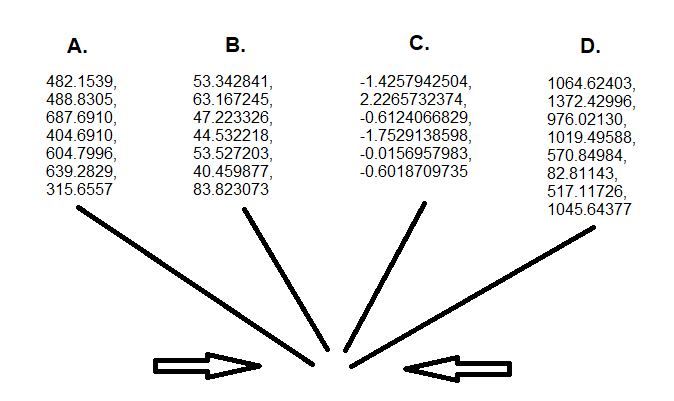
# I went ahead and sampled a few of the elements from each series which were generated by my system  #

testA <- c(482.154, 488.831, 687.691, 404.691, 604.8, 639.283, 315.656)

testB <- c(53.342841, 63.167245, 47.223326, 44.532218, 53.527203, 40.459877, 83.823073)

testC <-c(-1.4257942504, 2.2265732374, -0.6124066829, -1.7529138598, -0.0156957983, -0.6018709735 )

testD <- c(1064.62403, 1372.42996, 976.02130, 1019.49588, 570.84984, 82.81143, 517.11726, 1045.64377)

# We now must create a series which contains all of the sample elements #

testall <- c(testA, testB, testC, testD)

# Then we will take the mean measurement of each sampled series #

MLEA <- mean(testA)

MLEB <- mean(testB)

MLEC <- mean(testC)

MLED <- mean(testD)

# Next, we will derive the mean of the combined sample elements #

p_ <- mean(testall)

# We must assign to ‘N’, the number of sets which we are assessing #

N <- 4

# We must also derive the median of the combined sample elements #

medianden <- median(testall)

# Sigma2 = mean(testall) * (1 – (mean(testall)) / medianden #

sigma2 <- p_ * (1-p_) / medianden

# Now we’re prepared to calculate the assumed population mean of each sample series #

c_A <- p_+(1-((N-3)*sigma2/(sum((MLEA-p_)^2))))*(MLEA-p_)

c_B <- p_+(1-((N-3)*sigma2/(sum((MLEB-p_)^2))))*(MLEB-p_)

c_C <- p_+(1-((N-3)*sigma2/(sum((MLEC-p_)^2))))*(MLEC-p_)

c_D <- p_+(1-((N-3)*sigma2/(sum((MLED-p_)^2))))*(MLED-p_)

##################################################################################

# Predictive Squared Error #

PSE1 <- (c_A - 500) ^ 2 + (c_B - 50) ^ 2 + (c_C - 1) ^ 2 + (c_D - 1000) ^ 2

########################

# Predictive Squared Error #

PSE2 <- (MLEA- 500) ^ 2 + (MLEB - 50) ^ 2 + (MLEC - 1) ^ 2 + (MLED - 1000) ^ 2

########################

1 - 28521.5 / 28856.74

##################################################################################

1 - 28521.5 / 28856.74 = 0.01161739

So, we can conclude, through the utilization of MSE as an accuracy assessment technique, that Stein’s Methodology (AKA The James-Stein Estimator), provided a 1.16% better estimation of the population mean for each series, as compared to the mean of each sample series assessed independently.

Charles Stein really was a pioneer in the field of statistics as he discovered one of the first instances of dimension reduction.

If we consider our example data sources below: 


Applying the James-Stein Estimator to the data samples from each series’ source, removes the innate distance which exist between each sample. In simpler terms, this essentially equates to all elements within each sample being shifted towards a central point.


Series elements which were already in close proximity to the mean, now move slightly closer to the mean. Series elements which were originally far from the mean, move much closer to the mean. These outside elements still maintain their order, but they are brought closer to their fellow series peers. This shifting of the more extreme elements within a series, is what makes the James-Stein Estimator so novel in design, and potent in application.

This one really blew my noggin when I first discovered and applied it.

For more information on this noggin blowing technique, please check out:

https://www.youtube.com/watch?v=cUqoHQDinCM


That's all for today.

Come back again soon for more perspective altering articles.

-RD

Friday, October 28, 2022

(Python) The Number: 13 (Happy, Lucky, Primes) - A Spooky Special!

This Halloween, we’ll be covering a very spooky topic. 

I feel that the number “13”, for far too long, has been un-fairly maligned.

Today, it will have its redemption.

Did you know that the number “13”, by some definitions, is both a happy and lucky number? Let’s delve deeper into each definition, and together discover why this number deserves much more respect than it currently receives.

Happy Numbers
 
In number theory, a happy number is a number which eventually reaches 1 when replaced by the sum of the square of each digit. * 

Example:   

For instance, 13 is a happy number because:

(1 * 1) + (3 * 3) = 10

(1 * 1) + (0 * 0) = 1

and the number 19 is also a happy number because:

(1 * 1) + (9 * 9) = 82

(8 * 8) + (2 * 2) = 68

(6 * 6) + (8 * 8) = 100

(1 * 1) + (0 * 0) + (0 * 0) = 1

*- https://en.wikipedia.org/wiki/Happy_number

Lucky Numbers

In number theory, a lucky number is a natural number in a set which is generated by a certain "sieve". *

In the case of our (lucky) number generation process, we will be utilizing the, "the sieve of Josephus Flavius".


Example:

Beginning with a list of integers from 1 – 20:

{1, 2, 3, 4, 5, 6, 7, 8, 9, 10, 11, 12, 13, 14, 15, 16, 17, 18, 19, 20}

We will remove all even numbers:

1, 2, 3, 4, 5, 6, 7, 8, 9, 10, 11, 12, 13, 14, 15, 16, 17, 18, 19, 20

Leaving:

1, 3, 5, 7, 9, 11, 13, 15, 17, 19

The first remaining number after the number “1”, is the number “3”. Therefore, every third number within the list must be removed:

1, 3, 5, 7, 9, 11, 13, 15, 17, 19

Leaving:

1, 3, 7, 9, 13, 15, 19

Next, we will remove each seventh entry within the remaining list, as the number “7” is the value which occurs subsequent to “3”:

1, 3, 7, 9, 13, 15, 19

Leaving:

1, 3, 7, 9, 13, 15

If we were to continue with this process, each ninth entry which would also be subsequently removed from the remaining list, as the number “9” is the number which occurs subsequent to “7”. Since only 6 elements remain from our initial set, the process ends here.

We can then conclude, that the following numbers are indeed lucky:

1, 3, 7, 9, 13, 15

*- https://en.wikipedia.org/wiki/Lucky_number 

Prime Numbers

A prime number is a natural number greater than 1 that is not a product of two smaller natural numbers. *

13 fits this categorization, as it can only be factored down to a product of 13 and 1.

*- https://en.wikipedia.org/wiki/Prime_number

(Python) Automating the Process

Now that I have hopefully explained each concept in an understandable way, let’s automate some of these processes.

Happy Numbers

# Create a list of happy numbers between 1 and 100 #

# https://en.wikipedia.org/wiki/Happy_number #

# This code is a modified variation of the code found at: #

# https://www.phptpoint.com/python-program-to-print-all-happy-numbers-between-1-and-100/ #


# Python program to print all happy numbers between 1 and 100 #


# isHappyNumber() will determine whether a number is happy or not #

def isHappyNumber(num):

    rem = sum = 0;


# Calculates the sum of squares of digits #

    while(num > 0):

        rem = num%10;

        sum = sum + (rem*rem);

        num = num//10;

    return sum;


# Displays all happy numbers between 1 and 100 #     

print("List of happy numbers between 1 and 100: \n 1");


# for i in range(1, 101):, always utilize n+1 as it pertains to the number of element entries within the set #

# Therefore, for our 100 elements, we will utilize 101 as the range variable entry #


for i in range(1, 101):

    result = i;


    while(result != 1 and result != 4):

        result = isHappyNumber(result);

        if(result == 1):

            print(i);


Console Output:

List of happy numbers between 1 and 100:
1
7
10
13
19
23
28
31
32
44
49
68
70
79
82
86
91
94
97
100


# Code which verifies whether a number is a happy number #

# Code Source: # https://en.wikipedia.org/wiki/Happy_number #

# This process is unfortunately two steps # 


def pdi_function(number, base: int = 10):

    """Perfect digital invariant function."""

    total = 0

    while number > 0:

        total += pow(number % base, 2)

        number = number // base

return total


def is_happy(number: int) -> bool:

    """Determine if the specified number is a happy number."""

    seen_numbers = set()

    while number > 1 and number not in seen_numbers:

        seen_numbers.add(number)

        number = pdi_function(number)

    return number == 1


# First, we must run the initial function on the number in question #

# This function will calculate the number’s perfect digital invariant value #

# Example, for 13 #


pdi_function(13)

Console Output:

10

# The output value of the first function must then be input into the subsequent function, in order to determine whether or not the tested value (ex. 13) can appropriately be deemed “happy”. #

is_happy(10)


Console Output:

True


Lucky Numbers

# https://en.wikipedia.org/wiki/Lucky_number #

# The code below will determine whether or not a number is "lucky", as defined by the above definition of the term #

# The variable ‘number check’, must be set equal to the number which we wish to assess  #

number_check = 99


# Python code to convert list of #

# string into sorted list of integer #

# https://www.geeksforgeeks.org/python-program-to-convert-list-of-integer-to-list-of-string/ #


# List initialization

list_int = list(range(1,(number_check + 1),1))


# mapping

list_string = map(str, list_int)


# Printing sorted list of integers

numbers = (list(list_string))


# https://stackoverflow.com/questions/64956140/lucky-numbers-in-python #


def lucky_numbers(numbers):

    index = 1

    next_freq = int(numbers[index])

    while int(next_freq) < len(numbers):

        del numbers[next_freq-1::next_freq]

        print(numbers)

        if str(next_freq) in numbers:

            index += 1

            next_freq = int(numbers[index])

else:

    next_freq = int(numbers[index])

return


lucky_numbers(numbers)


Console Output:

['1', '3', '5', '7', '9', '11', '13', '15', '17', '19', '21', '23', '25', '27', '29', '31', '33', '35', '37', '39', '41', '43', '45', '47', '49', '51', '53', '55', '57', '59', '61', '63', '65', '67', '69', '71', '73', '75', '77', '79', '81', '83', '85', '87', '89', '91', '93', '95', '97', '99']

['1', '3', '7', '9', '13', '15', '19', '21', '25', '27', '31', '33', '37', '39', '43', '45', '49', '51', '55', '57', '61', '63', '67', '69', '73', '75', '79', '81', '85', '87', '91', '93', '97', '99']

['1', '3', '7', '9', '13', '15', '21', '25', '27', '31', '33', '37', '43', '45', '49', '51', '55', '57', '63', '67', '69', '73', '75', '79', '85', '87', '91', '93', '97', '99']

['1', '3', '7', '9', '13', '15', '21', '25', '31', '33', '37', '43', '45', '49', '51', '55', '63', '67', '69', '73', '75', '79', '85', '87', '93', '97', '99']

['1', '3', '7', '9', '13', '15', '21', '25', '31', '33', '37', '43', '49', '51', '55', '63', '67', '69', '73', '75', '79', '85', '87', '93', '99']

['1', '3', '7', '9', '13', '15', '21', '25', '31', '33', '37', '43', '49', '51', '63', '67', '69', '73', '75', '79', '85', '87', '93', '99'] 


The output of this function returns a series of numbers up to and including the number which is being assessed. Therefore, from this function's application, we can conclude that the following numbers are "lucky":


['1', '3', '7', '9', '13', '15', '21', '25', '31', '33', '37', '43', '49', '51', '63', '67', '69', '73', '75', '79', '85', '87', '93', '99'] 

(Only consider the final output as valid, as all other outputs are generated throughout the reduction process)

Prime Numbers

# The code below is rather self-explanatory #


# It is utilized to generate a a list of prime numbers included within the range() function # 

# Source: https://stackoverflow.com/questions/52821002/trying-to-get-all-prime-numbers-in-an-array-in-python #

checkMe = range(1, 100)

primes = []

for y in checkMe[1:]:

    x = y

    dividers = []

    for x in range(2, x):

        if (y/x).is_integer():

            dividers.append(x)

if len(dividers) < 1:
    
    primes.append(y)

print("\n"+str(checkMe)+" has "+str(len(primes))+" primes")

print(primes)

Console Output:

range(1, 100) has 25 primes
[2, 3, 5, 7, 11, 13, 17, 19, 23, 29, 31, 37, 41, 43, 47, 53, 59, 61, 67, 71, 73, 79, 83, 89, 97]


Conclusion


Having performed all of the previously mentioned tests and functions, I hope that you have been provided with enough adequate information to reconsider 13's unlucky status. Based upon my number theory research, I feel that enough evidence exists to at least relegate the number 13 to the status of "misunderstood".


13 isn't to be feared or avoided. It actually shares unique company amongst other "Happy Primes":


7, 13, 19, 23, 31, 79, 97, 103, 109, 139, 167, 193, 239, 263, 293, 313, 331, 367, 379, 383, 397, 409, 487


Even intermingling with the company of "Lucky Primes":


3, 7, 13, 31, 37, 43, 67, 73, 79, 127, 151, 163, 193, 211, 223, 241, 283, 307, 331, 349, 367, 409, 421, 433, 463, 487


And being a member of the very exclusive group, the "Happy Lucky Primes":


7, 13, 31, 79, 193, 331, 367, 409, 487


----------------------------------------------------------------------------------------------------------------------------- 

I wish you all a very happy and safe holiday.


I'll see you next week with more (non-spooky) content!


-RD

Monday, October 24, 2022

(Python) Machine Learning – Keras – Pt. V

Throughout the previous articles, we thoroughly explored the various machine learning techniques which employ tree methodologies as their primary mechanism. We also discussed the evolution of machine learning techniques, and how gradient boosting eventually came to overtake the various forest models as the preferred standard. However, the gradient boosted model was soon replaced by the Keras model. The latter still remains the primary method of prediction at this present time.

Keras differs from all of the other models in that it does not utilize the tree or forest methodologies as its primary mechanism of prediction. Instead, Keras employs something similar to a binary categorical method, in that, an observation is fed through the model, and at each subsequent layer prior to the output, Keras decides what the observation is, and what the observation is not. This may sound somewhat complicated, and in all manners, it truly is. However, what I am attempting to illustrate will become less opaque as you continue along with the exercise.

A final note prior to delving any further, Keras is a member of a machine learning family known as deep learning. Deep learning can essentially be defined as an algorithmic analysis of data which can evaluate non-linear relationships. This analysis also provides dynamic model re-calibration throughout the modeling process.

Keras Illustrated

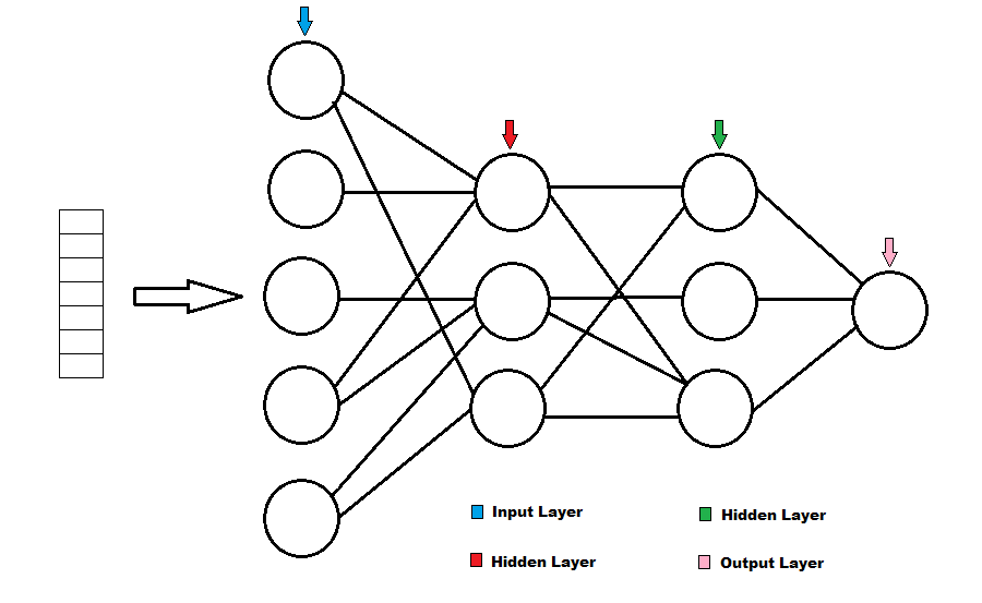
Below is a sample illustration of a Keras model which possesses a continuous dependent variable. The series of rows on the left represents the observational data which will be sent through the model so that it may “learn”. Each circle represents what is known as “neuron”, and each column of circles represents what is known as a “layer”. The sample illustration has 4 layers. The leftmost layer is known as the input layer, the middle two layers are known as the hidden layers, and the rightmost layer is referred to as the output layer.


Due to the model’s continuous dependent variable classification, it will only possess a single output layer. If the dependent variable was categorical, it would have an appearance similar to the graphic below:


How the Model Works

Without getting overly specific, (as many other resources exist which provide detailed explanations as it pertains the model’s inner-most mechanisms), the training of the model occurs throughout two steps. The first step being: “Forward Propagation”, and the second step being: “Backward Propagation”. Each node which exists beyond the input layers, sans the output layer, is measuring for a potential interaction amongst variables.

Each node is initially assigned a value. Those values shift as training data is processed through the model from the left to the right (forward propagation), and further, but more specifically modified, as the same data is then passed back through the model from the right to the left (back propagation). The entire training data set is not processed in its entirety in a simultaneous manner, instead, for the sake of allocating computing resources, the data is split into smaller sets known as batches. Batch size impacts learning significantly. With a smaller batch size, a model’s predictive capacity will be hindered. However, there are certain scenarios when lower batch size is advantageous, as the impact of noisy gradients will be reduced. The default size for a batch is 32 observations.

In many ways, the method in which the model functions is analogous to the way in which a clock operates. Each training observation shifts a certain aspect of a neuron’s value, with the neuron’s final value being representational of all of the prior shifts.

A few other terms which are also worth mentioning, as the selection of such is integral to model creation are:

Optimizer – This specifies the algorithm which will be utilized for correcting the model as errors occur.

Epoch – This indicates the number of times in which observational data will be passed through a model during the training process.

Loss Function – This indicates the algorithm which will be utilized to determine how errors are penalized within the model.

Metric - A metric is a function which is utilized to assess the performance of a model. However, unlike the Loss Function, it does not impact model training, and is only utilized to perform post-hoc analysis.

Model Application

As with any auxiliary python library, a library must first be downloaded and enabled prior to its utilization. To achieve this within the Jupyter Notebook platform, we will employ the following lines of code:

# Import ‘pip’ to import to install auxiliary packages #

import pip

# Install ‘TensorFlow’ to act as the underlying mechanism of the Keras UI #

pip.main(['install', 'TensorFlow'])

# Import pandas to enable data frame utilization #

import pandas

# Import numpy to enable numpy array utilization #

import numpy

# Import the general Keras library #

import keras

# Import tensorflow to act as the ‘backend’ #

import tensorflow

# Enable option for categorical analysis #

from keras.utils import to_categorical

from keras.models import Sequential

from keras.layers import Activation, Dense

# Import package to enable confusion matrix creation #

from sklearn.metrics import confusion_matrix

# Enable the ability to save and load models with the ‘load_model’ option #

from keras.models import load_model

# Enable the creation of confusion matrixes with the ‘sklearn.metrics’ library #

from sklearn.metrics import confusion_matrix


With all of the appropriate libraries downloaded and enabled, we can begin building our sample model.

Categorical Dependent Variable Model

For the following examples, we will be utilizing a familiar data set, the “iris” data set, which is available within the R platform.

# Import the data set (in .csv format), as a pandas data frame #

filepath = "C:\\Users\\Username\\Desktop\\iris.csv"

iris = pandas.read_csv(filepath)


First we will randomize the observations within the data set. Observational data should always be randomized prior to model creation.

# Shuffle the data frame #

iris = iris.sample(frac=1).reset_index(drop=True)


Next, we will remove the dependent variable entries from the data frame and modify the structure of the new data frame to consist only of independent variables.

predictors = iris.drop(['Species'], axis = 1).as_matrix()

Once this has been achieved, we must modify the variables contained within the original data set so that the categorical outcomes are designated by integer values.

This can be achieved through the utilization of the following code:

# Modify the dependent variable so that each entry is replaced with a corresponding integer #

from pandasql import *

pysqldf = lambda q: sqldf(q, globals())

q = """

SELECT *,

CASE

WHEN (Species = 'setosa') THEN '0'

WHEN (Species = 'versicolor') THEN '1'

WHEN (Species = 'virginica') THEN '2'

ELSE 'UNKNOWN' END AS SpeciesNum

from iris;

"""

df = pysqldf(q)

print(df)

iris0 = df


Next, we must make a few further modifications.

First, we must modify the dependent variable type to integer.

After such, we will identify this variable as being representative of a categorical outcome.

# Modify the dependent variable type from string to integer #

iris0['SpeciesNum'] = iris0['SpeciesNum'].astype('int')

# Modify the variable type to categorical #

target = to_categorical(iris0.SpeciesNum)


We are now ready to build our model!

# We must first specify the model type #

model = Sequential()

# Next, we will specify the output dimensions. This value will typically be [1] unless you are working with images. #

n_cols = predictors.shape[1]

# This next line specifies the traits of the input layer #

model.add(Dense(100, activation = 'relu', input_shape = (n_cols, )))

# This line specifies the traits of the hidden layer #

model.add(Dense(100, activation = 'relu'))

# This line specifies the traits of the output layer #

model.add(Dense(3, activation = 'softmax'))

# Compile the model by adding the optimizer, the loss function type, and the metric type #

# If the model’s dependent variable is binary, utilize the ‘binary_crossentropy' loss function #

model.compile(optimizer = 'adam', loss='categorical_crossentropy',

metrics = ['accuracy'])


With our model created, we can now go about training it with the necessary information.

As was the case with prior machine learning techniques, only a portion of the original data frame will be utilized to train the mode.

model.fit(predictors[1:100,], target[1:100,], shuffle=True, batch_size= 50, epochs=100)

With the model created, we can now test its effectiveness by applying it to the remaining data observations.

# Create a data frame to store the un-utilized observational data #

iristestdata = iris0[101:150]

# Create a data frame to store the model predictions for the un-utilized observational data #

predictions = model.predict_classes(predictors[101:150])

# Create a confusion matrix to assess the model’s predictive capacity #

cm = confusion_matrix(iristestdata['SpeciesNum'], predictions)

# Print the confusion matrix results to the console output window #

print(cm)


Console Output:

[[16    0    0]
[    0  17    2]
[    0    0   14]] 

Continuous Dependent Variable Model

The utilization of differing model types is necessitated by the scenario that each situation dictates. As was the case with previous machine learning methodologies, the Keras package also contains functionality which allows for continuous dependent variables types.

The steps for applying this model methodology are as follows:

# Import the 'iris' data frame #

filepath = "C:\\Users\\Username\\Desktop\\iris.csv"

iris = pandas.read_csv(filepath)

# Shuffle the data frame #

iris = iris.sample(frac=1).reset_index(drop=True)


In the subsequent lines of code, we will first identify the model’s dependent variable ‘Sepal.Length’. This variable, and its corresponding observations will be held within the new variable ‘iris0’. Next, we will create the variable, ‘predictors’. This variable will be comprised of all of the variables contained within the ‘iris0’ data frame, with the exception of the ‘Sepal.Length’ variable. The new data frame will stored within a matrix format. Finally, we will again define the ‘n_cols’ variable.

target = iris['Sepal.Length']

# Drop Species Name #

iris0 = iris.drop(columns=['Species'])


# Drop Species Name #

predictors = iris0.drop(['Sepal.Length'], axis = 1).as_matrix()

n_cols = predictors.shape[1]


We are now ready to build our model!

# We must first specify the model type #

modela = Sequential()

# Next, we will specify the output dimensions. This value will typically be [1] unless you are working with images. #

n_cols = predictors.shape[1]

# This next line specifies the traits of the input layer #

modela.add(Dense(100, activation = 'relu', input_shape=(n_cols,)))

# This line specifies the traits of the hidden layer #

modela.add(Dense(100, activation = 'relu'))

# This line specifies the traits of the output layer #

modela.add(Dense(1))

# Compile the model by adding the optimizer and the loss function type #

modela.compile(optimizer = 'adam', loss='mean_squared_error')


With the model created, we must now train the model with the following code:

modela.fit(predictors[1:100,], target[1:100,], shuffle=True, epochs=100)

As was the case with the prior examples, we will only be utilizing a sample of the original data frame for the purposes of model training.

With the model created and trained, we can now test its effectiveness by applying it to the remaining data observations.

from sklearn.metrics import mean_squared_error

from math import sqrt

predictions = modela.predict(predictors)

rms = sqrt(mean_squared_error(target, predictions))

print(rms)

Model Functionality

In some ways, the Keras modeling methodology shares similarities with the hierarchal cluster model. The main differentiating factor being, in addition to the underlying mechanism, the dynamic aspects of the Keras model.

Each Keras neuron represents a relationship between independent data variables within the training set. These relationships exhibit macro phenomenon which may not be immediately observable within the context of the initial data. When finally providing an output, the model considers which macro phenomenon illustrated the strongest indication of identification. The Keras model still relies on generalities to make predictions, therefore, certain factors which are exhibited within the observational relationships are held in higher regard. This phenomenon is known as weighing, as each neuron is assigned a weight which is adjusted as the training process occurs.

The logistic regression methodology functions in a similar manner as it pertains to assessing variable significance. Again however, we must consider the many differentiating attributes of each model. In addition to weighing latent variable phenomenon, the Keras model is able to assess for non-linear relationships. Both attributes are absent within the aforementioned model, as logistic regression only assesses for linear relationships and can only provide values for variables explicitly found within the initial data set.

The sequential() model type, which was specified within the build process, is one of the many model options available within the Keras package. The sequential option differs from the other model types in that it creates a network in which each neuron within each layer, is connected to each neuron within each subsequent layer. 

 Other Characteristics of the Keras Model

Depending on the size of the data set which acted as the training data for the model, significant time may be required to re-generate a model after a session is terminated. To avoid this un-necessary re-generation process, functions exist which enable the saving and reloading of model information.

# Saving and Loading Model Data Requires #

from keras.models import load_model

# To save a model #

modelname.save("C:\\Users\\filename.h5")

# To load a model #

modelname = load_model("C:\\Users\\filename.h5")

It should be mentioned that as it pertains to Keras models, you do possess the ability to train existing models with additional data should the need the arise.

For instance, if we wished to train our categorical iris model (“model”) with additional iris data, we could utilize the following code:

model.fit(newpredictors[100:150,], newtargets[100:150,], shuffle=True, batch_size= 50, epochs=100)

There are errors which currently exist at the time of this article’s creation, which have yet to be resolved pertaining to learning rate fluctuation within re-loaded Keras models. Currently, a provisional fix has been suggested*, in which the "adam" optimizer is re-configured for re-loaded models. This re-configuring, while keeping all of the "adam" optimizer default configurations, significantly lowers the optimizer’s default learning rate. The purpose of this shift is to account for the differentiation in learning rates which occur in established models.

# Specifying Optimizer Traits Requires #

from keras import optimizers

# Re-configure Optimizer #

liladam = optimizers.adam(lr=0.00001, beta_1=0.9, beta_2=0.999, epsilon=None, decay=0.0, amsgrad=False)

# Utilize Custom Optimizer #

model.compile(optimizer = liladam, loss='categorical_crossentropy',

            metrics = ['accuracy'])


*Source - https://github.com/keras-team/keras/issues/2378

Graphing Models

As we cannot easily determine the innermost workings of a Keras model, the best method of visualization can be achieved by graphing the learning output.

Prior to training the model, we will modify the typical fitting function to resemble something similar to the lines of code below:

history = model.fit(predictors[1:100,], target[1:100,], shuffle=True, epochs= 110, batch_size = 100, validation_data =(predictors[100:150,] , target[100:150,]))

What this code enables, is the creation of the data variable “history”, in which, data pertaining to the model training process will be stored. “validation_data” is instructing the python library to assess the specified data within the context of the model after each epoch. This does not impact the learning process. The way in which this assessment will be analyzed is determined by the selection of the “meteric” option specified within the model.fit() function.

If the above code is initiated, the model will be trained. To view the categories in which the model training history was organized upon being saved within the “history” variable, you may utilize the following lines of code.

history_dict = history.history

history_dict.keys()


This produces the console output:

dict_keys(['val_loss', 'val_acc', 'loss', 'acc'])

To set the appropriate axis lengths for our soon to be produced graph, we will initiate the following line:

epochs = range(1, len(history.history['acc']) + 1)

If we are utilizing Jupyter Notebook, we should also modify the graphic output size:

plt.rcParams["figure.figsize"] = [16,9]

We are now prepared to create our outputs. The first graphic can be prepared with the following code:

# Plot training & validation accuracy values #

# (This graphic cannot be utilized to track the validation process of continuous data models) #

plt.plot(epochs, history.history['acc'], 'b', label = 'Training acc')

plt.plot(epochs, history.history['val_acc'], 'bo', color = 'orange', label = 'Validation acc')

plt.title('Training and validation accuracy')

plt.ylabel('Loss')

plt.xlabel('Epoch')

plt.legend(loc='upper left')

plt.show()


This produces the output:


Interpreting this Graphic

What this graphic is illustrating, is the level of accuracy in which the model predicts results. The solid blue line represents the data which was utilized to train the model, and the orange dotted line represents the data which is being utilized to test the model’s predictability. It should be evident that throughout the training process, the predictive capacity of the model improves as it pertains to both training and validation data. If a large gap emerged, similar to the gap which is observed from epoch # 20 to epoch # 40, we would assume that this divergence of data is indicative of “overfitting”. This term is utilized to describe a model which can predict training results accurately, but struggles to predict outcomes when applied to new data.

The second graphic can be prepared with the following code:

# Plot training & validation loss values

plt.plot(epochs, history.history['loss'], 'b', label = 'Training loss')

plt.plot(epochs, history.history['val_loss'], 'bo', label = 'Validation loss', color = 'orange')

plt.title('Training and validation loss')

plt.ylabel('Loss')

plt.xlabel('Epoch')

plt.legend(loc='upper left')

plt.show()


Interpreting this Graphic

This graphic is illustrates the improvement of the model over time. The solid blue line represents the data which was utilized to train the model, and the orange dotted line represents the data which is being utilized to test the model’s predictability. If a gap does not emerge between the lines throughout the training process, it is advisable to set the number of epochs to a figure which, after subsequent graphing occurs, demonstrates a flat plateauing of both lines.

Reproducing Model Training Results

If Keras is being utilized, and TensorFlow is the methodology selected to act as a “backend”, then the following lines of code must be utilized to guarantee reproductivity of results.

# Any number could be utilized within each function #

# Initiate the RNG of the general python library #

import random

# Initiate the RNG of the numpy package #

import numpy.random

# Set a random seed as it pertains to the general python library #

random.seed(777)

# Set a random seed as it pertains to the numpy library #

numpy.random.seed(777)

# Initiate the RNG of the tensorflow package #

from tensorflow import set_random_seed

# Set a random seed as it pertains to the tensorflow library #

set_random_seed(777)

Missing Values in Keras


Much like the previous models discussed, Keras has difficulties as it relates to variables which contain missing observational values. If a Keras model is trained on data which contains missing variable values, the training process will occur without interruption, however, the missing values will be analyzed under the assumption that they are representative of a measurement. Meaning, that the library will NOT automatically assume that the value is a missing value, and from such, estimate a place holder value based on other variable observations within the set.

To make assumptions for the missing values based on the process described above, we must utilize the imputer() function from the python library: “sklearn”. Sample code which can be utilized for this purpose can be found below:

from sklearn.preprocessing import Imputer

imputer = Imputer()

transformed_values = imputer.fit_transform(predictors)


Additional details pertaining to this function, its utilization, and its underlying methodology, can be found within the previous article: “(R) Machine Learning - The Random Forest Model – Pt. III”.

Having tested this method of variable generation on sets which I purposely modified, I can attest that its capability for achieving such is excellent. After generating fictitious placeholder values and then subsequently utilizing the Keras package to create a model, comparatively speaking, I saw no differentiation between the predicted results related to each individual set.

Early Stopping

There may be instances which necessitate the creation of a model that will be applicable to a very large data set. This essentially, in most cases, guarantees a very long training time. To help assist in shortening this process, we can utilize an “early stopping monitor”.

First, we must import the package related to this feature:

from keras import losses

Next we will create and define the parameters pertaining to the feature:

# If model improvement stagnates after 2 epochs, the fitting process will cease #

early_stopping_monitor = keras.callbacks.EarlyStopping(monitor='loss', patience = 2, min_delta=0, verbose=0, mode='auto', baseline=None, restore_best_weights=True)

Many of the options present within the code above are defaults. However, there are few worth mentioning.

monitor = ‘loss’ - This option is specifically instructing the function to monitor the loss value during each training epoch.

patience = 2 – This option is instructing the function to cease training if the loss value ceases to decline after 2 epochs.

restore_best_weights=True – This option is indicating to the function that the values which occurred prior to lack of loss within the training process, should be the last values applied as it pertains to model training. The subsequent training values will be discarded.

With the early stopping feature defined, we can add it to the training function below:

history = model.fit(predictors[101:150,], target[101:150,], shuffle=True, epochs=100, callbacks =[early_stopping_monitor], validation_data =(predictors[100:150,] , target[100:150,]))

Final Thoughts on Keras

In my final thoughts pertaining to the Keras model, I would like to discuss the pros and cons of the methodology. Keras is, without doubt, the machine learning model type which possesses the greatest predictive capacity. Keras can also be utilized to identify images, which is a feature that is lacking within most other predive models. However, despite these accolades, Keras does fall short in a few categories.

For one, the mathematics which act a mechanism for the model’s predicative capacity are incredibly complex. As a result of such, model creation can only occur within a digital medium. With this complexity comes an inability to easily verify or reproduce results. Additionally, creating the optimal model configuration as it pertains to the number of neurons, layers, epochs, etc., becomes almost a matter of personal taste. This sort of heuristic approach is negative for the field of machine learning, statistics, and science in general.

Another potential flaw relates to the package documentation. The website for the package is poorly organized. The videos created by researchers who attempt to provide instruction are also poorly organized, riddled with heuristic approach, and scuttled by a severe lack of awareness. It would seem that no single individual truly understands how to appropriately utilize all of the features of the Keras package. In my attempts to properly understand and learn the Keras package, I purchased the book, DEEP LEARNING with Python, written by the package’s creator, Francois Chollet. This book was also poorly organized, and suffered from the assumption that the reader could inherently understand the writer’s thoughts.

This being said, I do believe that the future of statistics and predictive analytics lies parallel with the innovations demonstrated within the Keras package. However, the package is so relatively new, that not a single individual, including the creator, has had the opportunity to utilize and document its potential. In this lies latent opportunity for the patient individual to prosper by pioneering the sparse landscape.

It is my opinion that at this current time, the application of the Keras model should be paired with other traditional statistical and machine learning methodologies. This pairing of multiple models will enable the user and potential outside researchers to gain a greater understanding as to what may be motivating the Keras model’s predictive outputs.